Anisotropic Structures - Theory and Design Strutture anisotrope: - PowerPoint PPT Presentation
International Doctorate in Civil and Environmental Engineering Anisotropic Structures - Theory and Design Strutture anisotrope: teoria e progetto Paolo VANNUCCI Lesson 6 - May 29, 2019 - DICEA - Universit a di Firenze 1 / 67 Topics of the
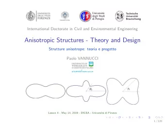
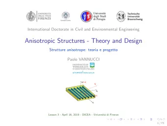
International Doctorate in Civil and Environmental Engineering Anisotropic Structures - Theory and Design Strutture anisotrope: teoria e progetto Paolo VANNUCCI Lesson 6 - May 29, 2019 - DICEA - Universit´ a di Firenze 1 / 67
Topics of the sixth lesson • A short introduction to laminated anisotropic structures - Part 2 • Some rules for the general design of laminates 2 / 67
Recall of some basic facts about laminates � � � h 2 � � � ε 0 N h A 2 B = , C = A − D . (1) h 2 h 3 M 2 B 12 D κ For identical plies, n n � � A = a k Q ( δ k ) , B = b k Q ( δ k ) , k =1 k =1 (2) n n � � C = c k Q ( δ k ) , D = d k Q ( δ k ) , k =1 k =1 where a k = 1 b k = 1 n , n 2 (2 k − n − 1) , c k = a k − d k , (3) d k = 1 n 3 [12 k ( k − n − 1) + 4 + 3 n ( n + 2)] , 3 / 67
x’ x = 3 3 x’ 2 With the polar formalism, we x 2 get θ x’ 1 x 1 n 0 = 1 T A � T 0 k ( z k − z k − 1 ) h k =1 n 1 = 1 � T A T 1 k ( z k − z k − 1 ) h k =1 → (4) A n 0 = 1 0 e 4 i Φ A � R 0 k e 4 i ( Φ 0 k + δ k ) ( z k − z k − 1 ) R A h k =1 n 1 = 1 1 e 2 i Φ A R A � R 1 k e 2 i ( Φ 1 k + δ k ) ( z k − z k − 1 ) h k =1 4 / 67
n 0 = 1 � T 0 k ( z 2 k − z 2 T B k − 1 ) h 2 k =1 n 1 = 1 T B � T 1 k ( z 2 k − z 2 k − 1 ) h 2 k =1 → (5) B n 0 = 1 0 e 4 i Φ B � R B R 0 k e 4 i ( Φ 0 k + δ k ) ( z 2 k − z 2 k − 1 ) h 2 k =1 n 1 = 1 1 e 2 i Φ B � R 1 k e 2 i ( Φ 1 k + δ k ) ( z 2 k − z 2 R B k − 1 ) h 2 k =1 5 / 67
n 0 = 4 � T 0 k ( z 3 k − z 3 T D k − 1 ) h 3 k =1 n 1 = 4 T D � T 1 k ( z 3 k − z 3 k − 1 ) h 3 k =1 → (6) D n 0 = 4 0 e 4 i Φ D � R D R 0 k e 4 i ( Φ 0 k + δ k ) ( z 3 k − z 3 k − 1 ) h 3 k =1 n 1 = 4 1 e 2 i Φ D � R 1 k e 2 i ( Φ 1 k + δ k ) ( z 3 k − z 3 R D k − 1 ) h 3 k =1 6 / 67
Some remarks: • the isotropic and anisotropic parts of all the tensors remain separated in the homogenization of the polar parameters, for all the tensors • it is immediately apparent that special orthotropies are preserved: R 0 k = 0 ∀ k ⇒ R A 0 = R B 0 = R C 0 = R D 0 = 0 (7) R 1 k = 0 ∀ k ⇒ R A 1 = R B 1 = R C 1 = R D 1 = 0 More results are obtained for laminates of identical plies ... 7 / 67
The polar method for the case of identical plies T A 0 = T 0 T A 1 = T 1 A → (8) 0 e 4 i Φ A R A 0 = R 0 e 4 i Φ 0 ( ξ 1 + i ξ 3 ) 1 e 2 i Φ A R A 1 = R 1 e 2 i Φ 1 ( ξ 2 + i ξ 4 ) T B 0 = 0 T B 1 = 0 B → (9) 0 e 4 i Φ B 0 = R 0 e 4 i Φ 0 ( ξ 5 + i ξ 7 ) R B 1 e 2 i Φ B 1 = R 1 e 2 i Φ 1 ( ξ 6 + i ξ 8 ) R B T D 0 = T 0 T D 1 = T 1 D → (10) 0 e 4 i Φ D 0 = R 0 e 4 i Φ 0 ( ξ 9 + i ξ 11 ) R D 1 e 2 i Φ D 1 = R 1 e 2 i Φ 1 ( ξ 10 + i ξ 12 ) R D 8 / 67
The polar method for the case of identical plies Lamination parameters (Tsai & Pagano, 1968) T A 0 = T 0 n T A 1 = T 1 a j e 4 i δ j ξ 1 + i ξ 3 = � A → (8) j =1 0 e 4 i Φ A R A 0 = R 0 e 4 i Φ 0 ( ξ 1 + i ξ 3 ) (11) n � a j e 2 i δ j ξ 2 + i ξ 4 = 1 e 2 i Φ A R A 1 = R 1 e 2 i Φ 1 ( ξ 2 + i ξ 4 ) j =1 T B 0 = 0 n b j e 4 i δ j � ξ 5 + i ξ 7 = T B 1 = 0 B → (9) j =1 (12) 0 e 4 i Φ B n 0 = R 0 e 4 i Φ 0 ( ξ 5 + i ξ 7 ) R B b j e 2 i δ j ξ 6 + i ξ 8 = � 1 e 2 i Φ B 1 = R 1 e 2 i Φ 1 ( ξ 6 + i ξ 8 ) R B j =1 n T D 0 = T 0 d j e 4 i δ j ξ 9 + i ξ 11 = � T D j =1 1 = T 1 (13) D → (10) n d j e 2 i δ j 0 e 4 i Φ D � 0 = R 0 e 4 i Φ 0 ( ξ 9 + i ξ 11 ) ξ 10 + i ξ 12 = R D j =1 1 e 2 i Φ D 1 = R 1 e 2 i Φ 1 ( ξ 10 + i ξ 12 ) R D 8 / 67
We then can see that for laminates of identical plies, all what has been said in the general case is still valid and in addition: • the isotropic part of A and D are identical to that of the basic layer • the isotropic part of B vanishes: B is merely anisotropic, with a null mean • hence, only the anisotropic part of the laminate can be tailored, while the choice of the basic layer automatically fixes the anisotropic part • this eliminates from the design problem the isotropic part, hence 6 design variables are eliminated 9 / 67
• another decomposition is obtained, that between material and geometric part • the first one is fixed once the basic layer chosen, and it is represented by the polar parameters of the basic layer • the second one is that to be designed, it accounts for the geometry of the laminate, i.e. orientation angles and stacking sequence, and is represented by the lamination parameters • to be remarked that this separation is possible only in the case of identical plies: the lamination parameters cannot be defined for hybrid laminates, but the polar parameters yes, they are universally valid, so they represent a more general concept and tool than that of lamination parameters • a question arises: can the lamination parameters, or, in the end, the mechanical parameters of the laminate, take any value? 10 / 67
Geometrical bounds The geometrical bounds (PV, J of Elas, 2013) replace, for laminates, the less strict thermodynamical bounds on elastic constants : laminates belong to a subset of the general elastic materials ρ = R L τ 0 = T L τ 1 = T L ρ 0 = R 0 ρ 1 = R 1 0 0 1 , , , , , c 0 = cos 4 Φ 0 . R L R L R L R L R L 1 0 1 0 1 ¡ 1 ¡ 1 ¡ 0 ≤ ρ 0 E E 0 ≤ ρ 1 ρ 1 ¡ ρ 1 ¡ ρ 0 ≤ 1 G G c 0 ¡ 1 ¡ 1 − ρ 2 0 ¡ c 0 ¡ 2 ρ 2 0 ρ 0 ¡ 1 ≤ 0 ¡ -‑1 ¡ ρ 0 ¡ 1 ¡ 1 ¡ 1 − ( − 1) K L ρ 0 c 0 Carbon-epoxy T-300/5208 Braided carbon-epoxy BR45-a 11 / 67
These bounds concern exclusively the polar parameters of A or D separately Nevertheless, these cannot be completely independent, because obtained as functions of the same quantities: the polar parameters of the basic layer and the orientation angles, besides the stacking sequence Hence, it should be preferable to establish the admissible set of all the laminate’s polar parameters This is still to be done and probably impossible to be obtained: previous studies on this subject, but done directly on the lamination parameters, so bounded only to the case of laminates of identical plies, never succeeded in solving this still open problem 12 / 67
This point constitutes one of the most serious mathematical open problems for a correct formulation of optimization problems of laminates including at the same time extension and bending properties For the while there are only two possibilities • to consider problems concerning only A or D ; this is what is commonly done, and usually only A is designed • to bound the research of the solution to the set of quasi-homogenous laminates; this approach is mathematically rigorous, because the admissible set of design variables is strictly the same for A and D . 13 / 67
Sensitivity to orientation errors • Errors always inexorably affect each quantity in practical realization. It is hence interesting to ponder what are the effects of such errors. • In the case of laminates, the most interesting error is that affecting ply orientations. About properties, different choices can be done. • A simple problem: which is the effect of an orientation error of a single layer on the coupling of a laminate designed to be uncoupled? (PV, J Elas, 2002) • The problem is stated introducing a suitable measure of the coupling and then analyzing the effects on it of an error on a single layer. The measure is the degree of coupling β defined as B β = B max , (14) where B is a suitable norm of B and B max is highest possible value. Of course, β ∈ [0 , 1] and β = 0 corresponds to uncoupling, while β = 1 to the highest possible coupling for the laminate. We take for B � 2 + 2 T B 2 + R B 2 + 4 R B 2 , B = T B (15) 0 1 0 1 14 / 67
For a laminate composed by identical layers � 2 + 4 R B 2 . R B B = (16) 0 1 With some standard passages we get � p � R 02 + 4 R 12 � � � b 2 � j + � � B = h 2 � j = − p � (17) � p p 2 � R 02 cos 4( δ l − δ m ) + 4 R 12 cos 2( δ l − δ m ) � � � � 2 b l b m � � l = − p m = l +1 To have B max the term p p 2 cos 4( δ l − δ m ) + 4 R 1 2 cos 2( δ l − δ m ) � � � � 2 (18) b l b m R 0 l = − p m = l +1 must be maximized (the rest depends on the basic layer). 15 / 67
Recommend
More recommend
Explore More Topics
Stay informed with curated content and fresh updates.
