Anisotropic Structures - Theory and Design Strutture anisotrope: - PowerPoint PPT Presentation
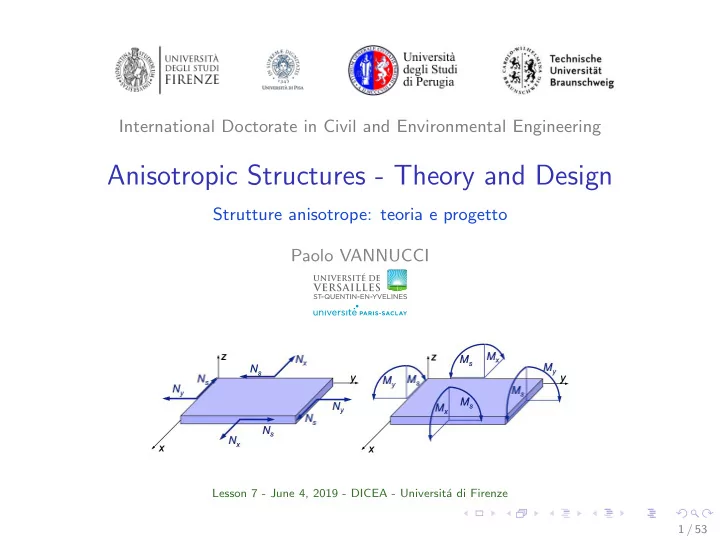
International Doctorate in Civil and Environmental Engineering Anisotropic Structures - Theory and Design Strutture anisotrope: teoria e progetto Paolo VANNUCCI Lesson 7 - June 4, 2019 - DICEA - Universit a di Firenze 1 / 53 Topics of the
International Doctorate in Civil and Environmental Engineering Anisotropic Structures - Theory and Design Strutture anisotrope: teoria e progetto Paolo VANNUCCI Lesson 7 - June 4, 2019 - DICEA - Universit´ a di Firenze 1 / 53
Topics of the seventh lesson • The design of anisotropic laminated structures as an optimization problem 2 / 53
About optimization techniques Because the design of laminated anisotropic structures is a difficult task, the basic idea is to transpose it into an effective, proved theory: that of mathematical optimization. In such a theoretical framework it is possible to give a correct and clear mathematical formulation of the design problems and also to find effective numerical tools for the resolution of such problems. Before going on, it is worth to recall some basic aspects of optimization theory and introduce some numerical tools particularly suited for the problems of laminates design. 3 / 53
Types of optimization problems Generally speaking, an optimization problem can be always reduced to a form of the type x i ∈ Ω f ( x i ) , min i = 1 , ..., n , (1) subjected to g j ( x i ) ≤ 0 , j = 1 , ..., p , and to h k ( x i ) = 0 , k = 1 , ..., q . with: • x i : design variables • f ( x i ): objective (or cost) function • g j ( x i ): inequality constraints • h k ( x i ): equality constraints The set Ω of the points x i that satisfy all the constraints is the feasible domain. 4 / 53
In several problems, a state equation is one of the equality constraints; it states a necessary condition to be satisfied by the solution, e.g. in mechanics the equilibrium equation, a condition that the optimal solution must satisfy (in some formulations, such a state equation can be put in variational form, for instance using the principle of minimum total potential energy, and it can enter directly the objective function, leading so to a double minimization problem). When there are more than one conflicting objectives to be minimized, the problem is multiobjective. A problem is continuous if x i ∈ R ∀ i = 1 , ..., n , discrete if ∃ i : x i / ∈ R . 5 / 53
Convexity Convexity is one of the most important characteristics of optimization problems. The reason is that convexity ⇒ uniqueness of the minimum. An optimization problem is convex ⇐ ⇒ the objective function f ( x i ) and the feasible domain Ω are convex. A domain Ω is convex ⇐ ⇒ ∀ x 1 , x 2 ∈ Ω , x 1 � = x 2 , x = (1 − t ) x 1 + t x 2 ∈ Ω ∀ t ∈ [0 , 1] . (2) The intersection of two or more convex domains is a convex domain. 6 / 53
A function f ( x i ) : Ω → R is convex on the convex domain Ω ⊂ R n ⇐ ⇒ ∀ x 1 , x 2 ∈ Ω , x 1 � = x 2 f ( λ x 1 + (1 − λ ) x 2 ) ≤ λ f ( x 1 ) + (1 − λ ) f ( x 2 ) ∀ λ ∈ (0 , 1) . (3) The function f ( x i ) is strictly convex if strict inequality holds. For n = 1, a convex function is below the line joining x 1 and x 2 . 3.3 A strictly convex ( left ), a convex ( middle ), and a nonconvex ( right ) function 7 / 53
Descent methods The basic idea for convex problems is to start from a given point and to go down until the minimum. Because the problem is convex, one arrives always to the minimum. � The descent methods make use of the derivatives of f ( x i ) ⇒ it can be used only with fonctions at least C 1 , so it cannot be used for ≤ discrete problems. = ∈ x R d’un � un 8 / 53
There are different descent methods; the basic one is the steepest descent method. It is composed of different steps: • choice of a feasible starting point x 0 i ∈ Ω; • for each step k , computation of the steepest descent direction d k i ; • for each step k , computation of the step length t k ; • calculation of the new point x k +1 = x k i + t k d k i . i • stop when d k i = 0 ∀ i . By the same properties of the gradient, d i = −∇ i f . The step length can be calculated by different methods: dichotomy, quadratic interpolation, golden section etc. 9 / 53
� � = + consécutives � x 1 t 0 d 0 x 3 t 1 d 1 x 0 x 2 It can be shown that d k · d k +1 = 0 → the method is not very effective. Other descent methods improve the descent track: quasi-Newton, conjugate gradient etc. Using descent methods with non-convex functions can lead to local minima: the starting point Q2 leads to the local minimum P2, while Q4 leads to the global minimum P4. 10 / 53
When constraints are imposed, the minimum can be on the boundary and it can corresponds to points where the gradient is not null. Different methods can be used to take into account for constraints: barrier, penalization etc. 11 / 53
Metaheuristics The true drawback of descent methods is the sensitivity to the initial point If the problem is non-convex, the convergence to a true global minimum is not guaranteed. To counter this problem, the basic idea is to work not with a unique point, but with a population of individuals. An individual is a vector x i , i = 1 , ..., n candidate to be a solution of the problem. Letting evolve a population of potential solutions help in reaching the global minimum. The dynamics that inspires the displacement of the population throughout the feasible domain is called a metaheuristic. 12 / 53
A metaheuristic is hence a rationale inspired by a given phenomenon that can be biological, social or physical. There are, in fact, several different metaheuristics: • simulated annealing, inspired by metallurgy of alloys; • ant colonies, inspired by the social dynamics of ants; • neural networks, inspired by the brain functioning; • tabu search, inspired by social rules; • genetic algorithms, inspired by Darwinian selection; • particle swarm optimization (PSO), inspired by the dynamics of flocks of birds or shoals of fishes. Metaheuristics are order zero methods: they do not need the calculation of the derivatives of the objective function. As such, they can be used also with discrete problems. 13 / 53
Genetic algorithms Genetic Algorithms (GAs) are perhaps the most used metaheuristic. GAs were introduced by Holland in 1965 and are inspired to the mechanism of natural selection (C. Darwin, The origin of species, 1859). The basic idea is that of letting evolve a population following the rules of the survival of the fittest (Darwinian selection). The dynamics of the changes of the population from a generation, i.e; an iteration of the algorithm, to the following one are based upon the laws of genetics. The success of GAs is mainly due to their robustness and effectiveness in dealing with non convex problems. 14 / 53
The general scheme of a classical GA is rather simple: Figure: General scheme of a classical GA 15 / 53
The adaptation of each individual is an operation aiming at giving a ranking of individuals with respect to the objective: better individuals, i.e. individuals for which the objective has a better value, have a better fitness ϕ . There are different ways to introduce a fitness, normally ϕ ∈ [0 , 1]: 0 corresponds to the worst individual, 1 to the fittest one. A classical way is to define the fitness as � c � f − min pop f ϕ = 1 + , c ≥ 1 . (4) min pop f − max pop f Coefficient c is used to tune the selection pressure. Defined in this way, 0 ≤ ϕ ≤ 1. 16 / 53
The Darwinian idea is that individuals with a better fitness, i.e. best adapted to environment, have a greater chance to survive a longer time, so to reproduce themselves. Hence, in the selection phase best fitted individuals have a greater chance to be selected. There are different ways to operate selection; in all the cases, a couple of individuals, the parents, is selected to be reproduced in the subsequent phases. Two widely used selection strategies are tournament and roulette wheel. 17 / 53
In the tournament selection, k individuals are randomly chosen and only the best one is selected; doing this N times, one gets N parents; these are then coupled randomly to generate N offsprings. In roulette wheel selection, N / 2 couples are randomly selected on the base of their fitness: the higher the fitness ϕ i of individual i , the higher its probability p i to be selected for reproduction: ϕ i = p i = . (5) � ∑ � N j =1 ϕ j = � la 12% 11% 9% 15% hasard, � 22% 23% 8% 35 18 / 53
Coding individuals: phenotypes and genotypes In a classical GA, each real or discrete variable, the phenotype, is coded binary to obtain its genotype. It is hence represented by a chain of 0s and 1s: the DNA chain of an individual. The genetic operations are done on the binary chains of two individuals, the parents, to obtain (hopefully) two better offsprings. There are two classical genetic operations: crossover and mutation. both of them are used to generate offsprings from selected parents; because of selection, there is a genetic improvement of the population, i.e., the objective function is globally improved. In this way, from a generation to the following one, more and more fitted individuals form the populations → the probability to have better individuals, i.e. phenotypes approaching the minimum, increases. 19 / 53
Genetic operations Classical binary operations are done on the genotypes, i.e. ont he binary strings. Cross-over on genes (1 gene=1 design variable) Cross-over allows to obtain 2 offsprings from two selected parents. The crossover point is randomly selected 20 / 53
Recommend
More recommend
Explore More Topics
Stay informed with curated content and fresh updates.
