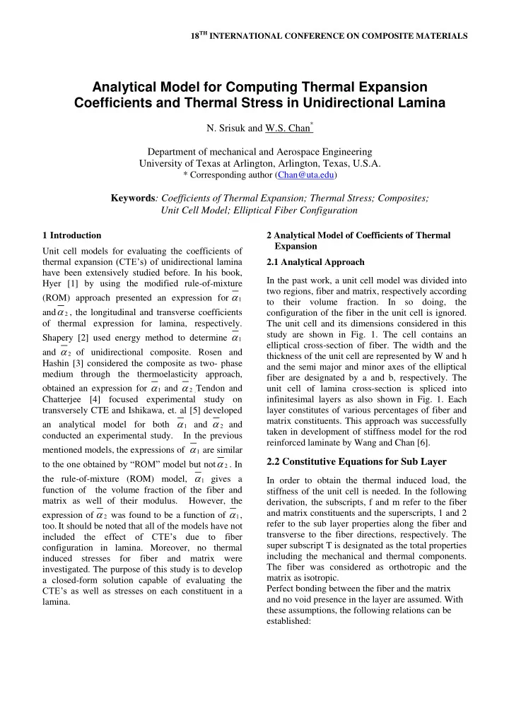
Analytical Model for Computing Thermal Expansion Coefficients and - PDF document

18 TH INTERNATIONAL CONFERENCE ON COMPOSITE MATERIALS Analytical Model for Computing Thermal Expansion Coefficients and Thermal Stress in Unidirectional Lamina N. Srisuk and W.S. Chan * Department of mechanical and Aerospace Engineering University of Texas at Arlington, Arlington, Texas, U.S.A. * Corresponding author (Chan@uta.edu) Keywords : Coefficients of Thermal Expansion; Thermal Stress; Composites; Unit Cell Model; Elliptical Fiber Configuration 1 Introduction 2 Analytical Model of Coefficients of Thermal Expansion Unit cell models for evaluating the coefficients of thermal expansion (CTE’s) of unidirectional lamina 2.1 Analytical Approach have been extensively studied before. In his book, In the past work, a unit cell model was divided into Hyer [1] by using the modified rule-of-mixture two regions, fiber and matrix, respectively according  (ROM) approach presented an expression for 1 to their volume fraction. In so doing, the  , the longitudinal and transverse coefficients and configuration of the fiber in the unit cell is ignored. 2 of thermal expression for lamina, respectively. The unit cell and its dimensions considered in this  study are shown in Fig. 1. The cell contains an Shapery [2] used energy method to determine 1 elliptical cross-section of fiber. The width and the  and of unidirectional composite. Rosen and 2 thickness of the unit cell are represented by W and h Hashin [3] considered the composite as two- phase and the semi major and minor axes of the elliptical medium through the thermoelasticity approach, fiber are designated by a and b, respectively. The  and  obtained an expression for . Tendon and unit cell of lamina cross-section is spliced into 1 2 infinitesimal layers as also shown in Fig. 1. Each Chatterjee [4] focused experimental study on transversely CTE and Ishikawa, et. al [5] developed layer constitutes of various percentages of fiber and   matrix constituents. This approach was successfully an analytical model for both and and 1 2 taken in development of stiffness model for the rod conducted an experimental study. In the previous reinforced laminate by Wang and Chan [6].  are similar mentioned models, the expressions of 1  . In 2.2 Constitutive Equations for Sub Layer to the one obtained by “ROM” model but not 2  the rule-of-mixture (ROM) model, gives a In order to obtain the thermal induced load, the 1 function of the volume fraction of the fiber and stiffness of the unit cell is needed. In the following matrix as well of their modulus. However, the derivation, the subscripts, f and m refer to the fiber  was found to be a function of  , and matrix constituents and the superscripts, 1 and 2 expression of 2 1 refer to the sub layer properties along the fiber and too. It should be noted that all of the models have not included the effect of CTE’s due to fiber transverse to the fiber directions, respectively. The super subscript T is designated as the total properties configuration in lamina. Moreover, no thermal including the mechanical and thermal components. induced stresses for fiber and matrix were The fiber was considered as orthotropic and the investigated. The purpose of this study is to develop matrix as isotropic. a closed-form solution capable of evaluating the Perfect bonding between the fiber and the matrix CTE’s as well as stresses on each constituent in a and no void presence in the layer are assumed. With lamina. these assumptions, the following relations can be established:

Fig. 1 Geometry and Dimension of Unit Cell Model Fig. 1 Geometry and Dimension of Unit Cell Model Q Q  22 22 (5) f m Q   (1) 22   Q Q V Q 22 m 22 f f 22 f Q Q  66 f 66 m Q     66 Q Q V Q 66 m 66 f f 66 f (2) The matrix of Q is defined as the same expression as given in most of the composite text such as in Ref. 1. (3) For each sub layer, the stress and strain relationships The fiber volume fraction, V f in each sub layer can are given as be written from the geometry of the fiber as       T       T Q Q 0 1 f  1 f 11 f 12 f      1 f     h h             T  0 z  , a   a ,     Q 0   T      2 2 2 f 22 f 2 f (4)  2 f         V   sym Q      r   2 12 f 66 f w 2 b z 12 f     i 1 z [ a a , ]   2   W W a     T  T      Q Q 0 m  1 m 11 m 12 m 1 m       (6)        T Q 0 T      where w i is the width of the fiber part of the i-th sub 2 m 22 m m       2 m  layer.        sym Q 12 m 66 m  12 m Substituting the stress/strain relationship for each       T constituent, the reduced stiffness matrix of the sub T      0 Q Q  1  1 11 12 1 layer can be written as              T     Q 0 T     2   2 2 22  2  V V Q Q        2 f     f f 12 m 12 f   Q Q Q V Q         sym Q 11 11 f 11 m f 11 m   12 66  Q Q V Q 12 22 m 22 f f 22 f     Q Q Q Q V Q Q It is also noted that thermal strain for the shear  12 f 22 m 12 m 22 f f 12 m 22 f Q     12 component is zero. Q Q V Q 22 m 22 f f 22 f

PAPER TITLE 2.3 CTE’s for Sub Layer The CTE’s can be obtained from mid -plane strains,  and  as shown below: 0 0 Substituting equation 1through 3 into 6 , we obtain α 1 1 2   and α 2 of each sub layer as expressed below: 0 0       1 2 and (10) 1 2  T T Q C Q C   22 1 12 2  and  can be obtained from the thermal 0 0  Where 1 2 Q Q Q 1 2 11 22 12 induced load as shown.  Q C Q C   11 2 12 1 (7)  2 2 Q Q Q    0 Th Th a N a N 11 22 12 1 11 x 12 x    0 Th Th a N a N (11) Where C 1 and C 2 are given as 2 12 x 22 x              V 1 V Q Q Q Q Q Q  f f 12 m 12 f 12 f 1 f 22 f 2 f 12 m m 22 m m The explicit expression of the lamina compliance C   1   Q Q V Q matrix, [a] was derived in Ref. 7. 22 m 22 f f 22 f                 V Q Q Q Q Q Q f 11 f 1 f 12 f 2 f 11 m m 12 m m 11 m m 12 m m 2.5 Thermal Stress of Fiber and Matrix of Lamina             V 1 Q Q Q Q Q  f 22 F 12 f 1 f 22 f 2 f 12 m m 22 m m C   For any given point of z, the thermal stress can be 2   Q Q V Q 22 m 22 f f 22 f  and  T T obtained from equation (6). In doing so, 1 2  and  . 0 0     should be replaced by Q Q (8) 1 2 12 f 1 f 22 f 2 f 3 Present Model Validation By Finite 2.4 Thermal Induced Load of Unit Cell Element Method   Th N The thermal resultant in-plane forces,   and A three- dimensional finite element model using ANSY 11.0 program was developed. E-glass fiber   Th M moment,   of lamina due to the change of with circular cross-section and Epoxy 3501-6 matrix were used as an example to demonstrate the validity temperature can be obtained by integrating the of the analytical solution. The material constants are constituent equation through the thickness of cross- sectional area with no external force. In this study, taken from Ref. [8] as listed below: the fiber is assumed to be placed at its center of the E 1f = E 2f = E 3f =10.5x10 6 psi; unit cell. Hence, the thermal induced moment is G 12f = G 23f = G 13f =4.3x10 6 psi zero. With aid of Equation 7, the thermal induced ν 12f = ν 23f = ν 13f =0.23; load can be simplified as α 1f = α 2f = α 3f =2.8x10 -6 in/in/ 0 F E m = 0.62x10 6 psi;     Th N C  x  1 G m = 0.24x10 6 psi; ν m = 0.35; h       Th N T 2 C dz   (9)   y h 2      2 Th Solid95 of 20-node solid element with three degrees N  0    xy of freedom in each node was used. The dimension in It should be noted that C 1 and C 2 are a function of V f length and cross-section of the model used was 0.05 which is dependent of z. The detailed integration  and 0.0005 in x 0.005 in x 0.005 in x 0.005 in for was carried out in a closed form expression shown in 1  . The present results compared Ref. [7]. in x 0.005 in for 2 with the data given in Ref. [8] was in difference of  and 3 % for  . 2.5 Thermal Expansion Coefficients of 0.37% for 1 2 Lamina 3