Analysis of SNP Marker Data for Predictions Some remarks about - PowerPoint PPT Presentation

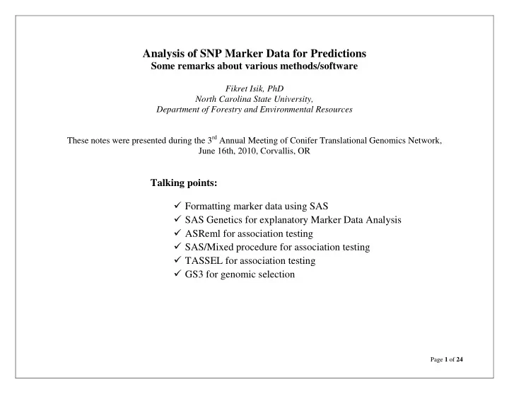
Analysis of SNP Marker Data for Predictions Some remarks about various methods/software Fikret Isik, PhD North Carolina State University, Department of Forestry and Environmental Resources These notes were presented during the 3 rd Annual Meeting of Conifer Translational Genomics Network, June 16th, 2010, Corvallis, OR Talking points:  Formatting marker data using SAS  SAS Genetics for explanatory Marker Data Analysis  ASReml for association testing  SAS/Mixed procedure for association testing  TASSEL for association testing  GS3 for genomic selection Page 1 of 24

Marker data  Marker data sets are typically very large.  For example, genotyping 2,000 trees for 10,000 SNP markers means 20 million data points. Assuming the markers are biallelic, 20,000 effects (covariates) need to be estimated. Data might be in very different formats, for example... tree18 tree19 tree 20 tree 21 tree 22 tree 23 tree 24 tree 25 ... GG GG GG GG GG GG GG GG GG 01-256 AC AA AA AA AA AA AA AA AA 01-71 01-559 CC CC CC CC CC CC CC CC CC 01-431 GG AG GG 0 GG AG GG AG AG ... GG GG GG 0 GG GG GG GG GG  The rows are marker IDs, usually long strings of text and numbers.  Tree 18 is homozygous (GG) for locus 01-256 but it is heterozygous (AC) for the second locus.  The 0 values are missing values. For some reason some trees were not genotyped (lack of enough DNA etc.)  Sometimes, there is no segregation for a marker in the genotyped population. For example, all the trees for marker 01-559 are homozygous CC genotypes.  Data might come in different formats from different labs/companies. For example, in the following data set, we have minor allele frequency in the locus for a given tree instead of genotype. If we assume A is the minor allele, then AA=0, AC/CA=1, CC=2. The columns are again locus ID. Page 2 of 24

0-16213-01-477 0-15220-02-63 2-2199-01-392 CL1651Contig1-03-58 1 1 1 1 1 1 1 1 1 1 1 1 1 1 1 1 1 1 1 1 1 1 1 1 1 1 1 1 1 1 1 1 1 1 1 1 1 1 1 1 1 1 1 1 1 1 1 1 1 1 1 1 1 1 2 2 1 1 2 1 1 1 1 1 1 0 1 0 0 1 1 1 0 2 0 0 0 0 0 0 1 0 1 0 0 0 1 0 0 0 0 1 0 1 1 0  When data are obtained, the first task is to summarize, change the format and organize data by comprehensive software. I am comfortable with SAS software since I have been using for two decades but you may use R or some others.  The SAS software is powerful to handle large and complicated marker data. The following code is used to read 2963 markers into SAS environment. /* Getting data into SAS */ data A; length clone $ 10 s1-s2963 $ 3 ; infile "&folder\PCdataAll_char.csv" delimiter=',' missover DSD lrecl= 4000 firstobs= 2 ; input clone $ (s1-s2963) ($) ; run ;  SAS Macro scripts are efficient to format data for different software. In the following table, each column is a SNP marker genotype as explained before (AA=0, AC/CA=1, CC=2) Obs a100 a101 a111 a112 a150 a151 a440 a441 1 1 1 1 1 1 1 1 0 2 1 1 0 0 1 1 0 1 3 1 1 1 1 0 1 0 1 4 1 1 1 1 1 1 0 0 Page 3 of 24

 A software called GS3 developed by Legarra and colleagues can be used to simultaneously predict the overall markers additive and dominance effect (genome-wide selection). The software requires a different format of data. The genotypes should be as follows: AA=11, AC/CA=12, CC=22. The following SAS script converts 3406 SNP marker loci genotypic classes (0, 1, 2) to format required by GS3 (11, 12, 22). data A (drop=i); set pc.alleles ; array svars $ a1-a3406; array gvars $ g1-g3406; do i= 1 to 3406 ; if not missing (svars[i]) then do; if svars[i] ='0' then gvars[i]='11'; if svars[i] ='1' then gvars[i]='12'; if svars[i] ='2' then gvars[i]='22'; end; end; run ;  The SAS data step below compile all the markers into one column and export as a text file. GS3 requires a solid (one column) of marker genotypes * Concatenate marker to create one dummy variable-No space between alleles; Data A ; set A ; file "&folder\SNPout2.txt" lrecl= 50500 ; put @ 1 mu @ 3 tree @ 8 lignin 5.2 @ 14 cellulose 5.2 + 4 @ ; array svars $ g1-g6812; do i= 1 to 6812 ; put svars[i] $2. @ ; end; put ; run ; Page 4 of 24

The OUTPUT data (text) is ready to analyze with GS3 and obtain the overall additive, dominance and total genetic effects of markers (predictions or breeding values of trees) mu tree trait1 trait2 SNP markers (3406 of them, no space) 1 1 26.57 41.53 121212121212121212121212121212121212 1 2 27.21 41.28 121212121212121212121212121212121212 1 3 27.45 40.30 121212121212121212121212121212121212 mu is a dummy variable needed to fit intercept in genome-wide selection models. SAS Genetics for Exploratory Marker Data Analysis The ALLELE procedure in SAS Genetics performs preliminary analyses on genetic marker data: 1. The frequency of homozygous and heterozygous markers, 2. Polymorphic info content (PIC) 3. If a marker is heterozygous, the minor allele frequency for each marker 4. Detect errors in genotyping 5. Test Hardy Weinberg Equilibrium for each marker  Such measures can be useful in determining which markers to use for further linkage or association testing with a trait. High values of heterozygosity or PIC statistics are a sign of marker informativeness, which is a desirable property in linkage and association tests. Page 5 of 24

 Proc Allele requires data in different formats to produce above statistics. For example, the procedure requires that the first two columns in the data contain the set of alleles at the first marker, the second two columns contain set of alleles at the second marker etc.  Alternatively the columns can be genotypes or one column per each marker. The following DATA step could be used to produce the desired format for 2963 alleles to summarize data using Proc ALLELE: data Genotype (drop = i); set A; array fixit {*} $ snp1 – snp2963; do i = 1 to dim(fixit); fixit(i) = catx("/",substr(fixit(i), 1 , 1 ),substr(fixit(i), 2 , 1 )); end; run ; Output tree snp1 snp2 snp3 snp4 snp5 snp6 ... A/A A/A A/C A/A A/C A/A 18 A/C A/A A/A A/A A/C A/A 19 A/C A/A A/C A/A A/C A/A 20 A/C A/A A/C A/A C/C A/A 21 ...  The following Proc ALLELE code computes descriptive statistics for 2963 markers using above data format. The code uses bootstrapping to come up with test statistics /*computing allele and genotype frequencies*/ proc allele data=genotype outstat=ld prefix=SNP Page 6 of 24

perms= 10000 boot= 1000 seed= 123 genocol delimiter='/'; var s1-s2963; run ; Marker summary Locus Number Number Polymorph Allelic HWE of of Info Diversity Pr > Indiv Alleles Content ChiSq SNP1 134 2 0.2178 0.2487 0.0280 SNP2 130 2 0.2947 0.3591 0.9394 SNP3 132 2 0.3666 0.4835 <.0001 SNP4 136 2 0.3749 0.4999 0.7334 SNP5 133 2 0.1893 0.2117 0.0008  In above output SNP4 is the most informative because of its high PIC values. The Chi-square tests of HWE suggest that the segregation of SNP marker is independent of trees in the population. The below table is showing the allele frequencies for 3 markers and the minor allele frequency (MAF) is highlighted for them. Allele Frequencies Locus Allele Count Frequency Std Err 95% Confidence Limits SNP1 A 229 0.8545 0.0235 0.8074 0.8985 0.1455 C 39 0.0235 0.1015 0.1926 SNP2 A 199 0.7654 0.0262 0.7099 0.8135 C 61 0.2346 0.0262 0.1865 0.2901 SNP3 A 156 0.5909 0.0238 0.5423 0.6402 C 108 0.4091 0.0238 0.3598 0.4577 Page 7 of 24

Marker-trait Associations using linear models SAS/MIXED procedure For a random mating population with no population structure we can use LS regression to test the association between a marker and a trait. y = 1 n  + X g + e where mu is the only fixed effect y = X  + e to include other fixed effects y is a vector of phenotypes, 1n is a vector of 1s, X is a design matrix, g is the fixed effect of the marker and e is a vector of random errors ~ NID (0, σ 2 e ). The null hypothesis (H0) is that the marker has no effect on the trait, while the alternative hypothesis (H1) is that the marker does affect the trait (because it is in LD with a QTL). We can use SAS, TASSEL, ASReml or some other software to test the association of each marker with the phenotype. Based on F-tests we can choose a subset of markers and use them in mixed models to predict breeding values of trees. We can create arrays in the data step of SAS to run repeated jobs. The following script creates array for 2963 SNP markers. /* Create array for SNPS */ data ds; set &ds; array SNP{ 2963 } SNP1-SNP2963; run ; Page 8 of 24

The MIXED procedure can run mixed models to account for fixed and random effects while testing the null hypothesis (H0: No association between the marker and trait). The following macro code fits a mixed model to 2963 SNP markers. %macro genoanova ; %do i= 1 %to 2963; title "SNP &i"; proc mixed data=ds noinfo; class SNP&i female; model phenotype = SNP&i ; random female /solution ; run; %end; %mend ; % genoanova In above code we get the F-tests for all the markers but also the solutions (best linear unbiased predicted GCA values) of female. The SOLUTIONS option in the code provides the solutions of mixed model equations (BLUP) for female effects. Type 3 Tests of Fixed Effects Num Den Effect DF DF F Value Pr > F SNP1 2 2791 2.07 0.1266 Some remarks about using SAS/Mixed procedure  Marker is fit as fixed effect but can be as random Page 9 of 24