ANALYSIS OF ALGORITHMS AND BIG-O CS16: Introduction to Algorithms - PowerPoint PPT Presentation
1 Tuesday, January 31, 2017 ANALYSIS OF ALGORITHMS AND BIG-O CS16: Introduction to Algorithms & Data Structures Tuesday, January 31, 2017 2 Outline 1) Running time and theoretical analysis 2) Big-O notation 3) Big- and Big- 4)
1 Tuesday, January 31, 2017 ANALYSIS OF ALGORITHMS AND BIG-O CS16: Introduction to Algorithms & Data Structures
Tuesday, January 31, 2017 2 Outline 1) Running time and theoretical analysis 2) Big-O notation 3) Big-Ω and Big-Θ 4) Analyzing Seamcarve runtime 5) Dynamic programming 6) Fibonacci sequence
Tuesday, January 31, 2017 3 What is an “Efficient” Algorithm? • Efficiency measures • Small amount of time? on a stopwatch? • Low memory usage? • Low power consumption? • Network usage? • Analysis of algorithms helps quantify this
Tuesday, January 31, 2017 4 Measuring Running Time • Experimentally 9000 8000 • Implement algorithm 7000 6000 • Run program with inputs of Time (ms) 5000 varying size 4000 • Measure running times 3000 2000 • Plot results 1000 0 0 50 100 • Why not? Input Size • What if you can’t implement algorithm? • Which inputs do you choose? • Depends on hardware, OS, …
Tuesday, January 31, 2017 5 Measuring Running Time • Grows with the input size • Focus on large inputs • Varies with input • Consider the worst-case input
Friday, January 28, 2014 6 Measuring Running Time • Why worst-case inputs? • Easier to analyze • Practical: what if autopilot was slower than predicted for some untested input? • Why large inputs? • Easier to analyze • Practical: usually care what happens on large data
Tuesday, January 31, 2017 7 Theoretical Analysis • Based on high-level description of algorithm • Not on implementation • Takes into account all possible inputs • Worst-case or average-case • Quantifies running time independently of hardware or software environment
Friday, January 28, 2014 8 Theoretical Analysis • Associate cost to elementary operations • Find number of operations as function of input size
Tuesday, January 31, 2017 9 Elementary Operations • Algorithmic “time” is measured in elementary operations • Math (+, -, *, /, max, min, log, sin, cos, abs, ...) • Comparisons ( ==, >, <=, ...) • Variable assignment • Variable increment or decrement • Array allocation • Creating a new object • Function calls and value returns • (Careful, object's constructor and function calls may have elementary ops too!) • In practice, all these operations take different amounts of time • In algorithm analysis assume each operation takes 1 unit of time
Tuesday, January 31, 2017 10 Example: Constant Running Time function first(array): // Input: an array // Output: the first element return array[0] // index 0 and return, 2 ops • How many operations are performed in this function if the list has ten elements? If it has 100,000 elements? • Always 2 operations performed • Does not depend on the input size
Tuesday, January 31, 2017 11 Example: Linear Running Time function argmax(array): // Input: an array // Output: the index of the maximum value index = 0 // assignment, 1 op for i in [1, array.length): // 1 op per loop if array[i] > array[index]: // 3 ops per loop index = i // 1 op per loop, sometimes return index // 1 op • How many operations if the list has ten elements? 100,000 elements? • Varies proportional to the size of the input list: 5n + 2 • We’ll be in the for loop longer and longer as the input list grows • If we were to plot, the runtime would increase linearly
Tuesday, January 31, 2017 12 Example: Quadratic Running Time function possible_products(array): // Input: an array // Output: a list of all possible products // between any two elements in the list products = [] // make an empty list, 1 op for i in [0, array.length): // 1 op per loop for j in [0, array.length): // 1 op per loop per loop products.append(array[i] * array[j]) // 4 ops per loop per loop return products // 1 op • About 5n 2 + n + 2 operations (okay to approximate!) • A plot of number of operations would grow quadratically! • Each element must be multiplied with every other element • Linear algorithm on previous slide had 1 for loop • This one has 2 nested for loops • What if there were 3 nested loops?
Tuesday, January 31, 2017 13 Summarizing Function Growth • For large inputs growth rate is less affected by: 1E+19 10 5 n 2 + 10 8 n Quadratic • constant factors Quadratic 1E+16 n 2 10n + 10 5 • lower-order terms Linear n 1E+13 Linear T(n) 1E+10 • Examples • 10 5 n 2 + 10 8 n and n 2 grow 1E+7 with same slope despite 1E+4 differing constants and lower- order terms 1E+1 • 10n + 10 5 and n both grow 1E+1 1E+3 1E+5 1E+7 n with same slope as well In this graph (log scale on both axes), the slope of a line corresponds to the growth rate of its respective function
Tuesday, January 31, 2017 14 Big-O Notation • Given any two functions f(n) and g(n) , we say that f(n) f( n) is O( O(g( g(n)) if there exist positive constants c and n 0 such that f( f(n) n) ≤ cg( cg(n) for all n n ≥ n 0 10,000 3n • Example: 2n + 10 is O(n) 2n+10 1,000 • Pick c = 3 and n 0 = 10 n 2n + 10 ≤ 3n 100 2(10) + 10 ≤ 3(10) 30 ≤ 30 10 1 n 1 10 100 1,000
Tuesday, January 31, 2017 15 Big-O Notation (continued) • Example: n 2 is not O(n) • n 2 ≤ cn • n ≤ c • The above inequality cannot be satisfied because c must be a constant, therefore for any n > c the inequality is false
Tuesday, January 31, 2017 16 Big-O and Growth Rate • Big-O gives upper bound on growth of function • An algorithm is O(g(n)) if growth rate is no more than growth rate of g(n) • n 2 is not O(n) • But n is O(n 2 ) • And n 2 is O(n 3 ) • Why? Because Big-O is an upper bound!
Tuesday, January 31, 2017 17 Summary of Big-O Rules • If f(n) is a polynomial of degree d then • f(n) is O(n d ) . • In other words • forget about lower-order terms • forget about constant factors • Use the smallest possible degree • True that 2n is O(n 50 ) , but that’s not helpful • Instead, say it’s O(n) • discard constant factor & use smallest possible degree
Tuesday, January 31, 2017 18 Constants in Algorithm Analysis • Find number of elementary operations executed as a function of input size • first : T(n) = 2 • argmax : T(n) = 5n + 2 • possible_products : T(n) = 5n 2 + n + 3 • In the future skip counting operations • Replace constants with c since irrelevant as n grows • first : T(n) = c • argmax : T(n) = c 0 n + c 1 • possible_products: T(n) = c 0 n 2 + n + c 1
Tuesday, January 31, 2017 19 Big-O in Algorithm Analysis • Easy to express T(n) in big-O • drop constants and lower-order terms • In big-O notation • first is O(1) • argmax is O(n) • possible_products is O(n 2 ) • Convention for T(n) = c is O(1)
Tuesday, January 31, 2017 20 Big-Omega (Ω) • Recall f(n) is O(g(n)) • if f(n) ≤ cg(n) for some constant as n grows • Big-O means f(n) grows no faster than g(n) • g(n) acts as upper bound to f(n) ’s growth rate • What if we want to express a lower bound? Big-Omega • We say f(n) is Ω(g(n)) if f(n) ≥ cg(n) • f(n) grows no slower than g(n)
Tuesday, January 31, 2017 21 Big-Theta ( Θ ) • What about an upper and lower bound? Big-Theta • We say f(n) is Θ(g(n)) if f(n) is O(g(n)) and Ω(g(n)) • f(n) grows the same as g(n) (tight-bound)
Tuesday, January 31, 2017 22 How fast is the seamcarve algorithm ? • How many seams in c×r image? • At each row, seam can go: Left, Right, Down • It chooses 1 out of 3 dirs at each row and there are r rows • So 3 r possible seams from some starting pixel • Since there are c starting pixels total seams is • c × 3 r • For square image with n total pixels • there are possible seams n × 3 n
Tuesday, January 31, 2017 23 Seamcarve • Algorithms that try every possible solution are known exhaustive algorithms or brute force algorithms • Exhaustive approach is to consider all n × 3 n seams and choose the least important • What would be the big-O running time? O ( n × 3 n ) : exponential and not good •
Tuesday, January 31, 2017 24 Seamcarve • What is runtime of the algorithm from last class? • Remember: constants don’t affect big-O runtime • The algorithm: • Iterate over all pixels from bottom to top • populate costs and dirs arrays • Create seam by choosing minimum value in top row and tracing downward • How many times do we evaluate each pixel? • A constant number of times • So algorithm is linear: O(n), n is number of pixels • Hint: we also could have looked at pseudocode and counted number of nested loops!
Tuesday, January 31, 2017 25 Seamcarve: Dynamic Programming • From exponential algorithm to a linear algorithm?!? • Avoided recomputing information we already calculated! • Many seams cross paths • we don’t need to recompute sums of importances if we’ve already calculated it before • That’s the purpose of the additional costs array • Storing computed information to avoid recomputing later, is called dynamic programming
Tuesday, January 31, 2017 26 Fibonacci: Recursive 0, 1, 1, 2, 3, 5, 8, 13, 21, 34, … • The Fibonacci sequence is defined by the recurrence relation: F 0 = 0, F 1 = 1 F n = F n-1 + F n-2 • This lends itself very well to a recursive function for finding the n th Fibonacci number function fib(n): if n = 0: return 0 if n = 1: return 1 return fib(n-1) + fib(n-2)
Recommend
More recommend
Explore More Topics
Stay informed with curated content and fresh updates.







![Specifications & Testing [Andersen, Gries, Lee, Marschner, Van Loan, White] Recall: The](https://c.sambuz.com/494236/specifications-testing-s.webp)