Analysis and Computation for Finance Time Series - An Introduction - PowerPoint PPT Presentation
ECMM703 Analysis and Computation for Finance Time Series - An Introduction Alejandra Gonz alez Harrison 161 Email: mag208@exeter.ac.uk Time Series - An Introduction A time series is a sequence of observations ordered in time;
ECMM703 Analysis and Computation for Finance Time Series - An Introduction Alejandra Gonz´ alez Harrison 161 Email: mag208@exeter.ac.uk
Time Series - An Introduction • A time series is a sequence of observations ordered in time; observations are numbers (e.g. measurements). • Time series analysis comprises methods that attempt to: – understand the underlying context of the data (where did they come from? what generated them?); – make forecasts (predictions). 1
Definitions/Setting • A stochastic process is a collection of random variables { Y t : t ∈ T } defined on a probability space (Ω , F , P ). • In time series modelling, a sequence of observations is considered as one realisation of an unknown stochastic process: 1. can we infer properties of this process? 2. can we predict its future behaviour? • By time series we shall mean both the sequence of observations and the process of which it is a realization (language abuse). • We will only consider discrete time series: observations ( y 1 , . . . , y N ) of a variable at different times ( y i = y ( t i ), say). 2
Setting (cont.) • We will only deal with time series observed at regular time points (days, months etc.). • We focus on pure univariate time series models: a single time series ( y 1 , . . . , y N ) is modelled in terms of its own values and their order in time. No external factors are considered. • Modelling of time series which: – are measured at irregular time points, or – are made up of several observations at each time point (multi- variate data), or – involve explanatory variables x t measured at each time point, is based upon the ideas presented here. 3
Work plan • We provide an overview of pure univariate time series models: – ARMA (‘Box-Jenkins’) models; – ARIMA models; – GARCH models. • Models will be implemented in the public domain general purpose statistical language R. 4
References 1. Anderson, O. D. Time series analysis and forecasting The Box- Jenkins approach . Butterworths, London-Boston, Mass., 1976. 2. Box, George E. P. and Jenkins, Gwilym M. Time series analysis: forecasting and control . Holden-Day, San Francisco, Calif. 1976 3. Brockwell, Peter J. and Davis, Richard A. Time series: theory and methods , Second Edition. Springer Series in Statistics, Springer- Verlag. 1991. 4. Jonathan D. Cryer Time series Analysis . PWS-KENT Publishing Company, Boston. 1986. 5. R webpage : http://cran.r-project.org 6. Time Series Analysis and Its Applications: With R Examples . http://www.stat.pitt.edu/stoffer/tsa2/R_time_series_quick_fix.html 5
Statistical versus Time series modelling Problem: Given a time series ( y 1 , y 2 , . . . , y N ) : (i) determine tem- poral structure and patterns; (ii) forecast non-observed values. Approach: Construct a mathematical model for the data. • In statistical modelling it is typically assumed that the observations ( y 1 , . . . , y N ) are a sample from a sequence of independent random variables. Then – there is no covariance (or correlation) structure between the observations; in other words, – the joint probability distribution for the data is just the product of the univariate probability distributions for each observation; – we are mostly concerned with estimation of the mean behaviour µ i and the variance σ 2 i of the error about the mean, errors being unrelated to each other. 6
Statistical vs. Time series modelling (cont.) • However, for a time series we cannot assume that the observations ( y 1 , y 2 , . . . , y N ) are independent: the data will be serially correlated or auto-correlated, rather than independent. • Since we want to understand/predict the data, we need to ex- plain/use the correlation structure between observations. • Hence, we need stochastic processes with a correlation structure over time in their random component. • Thus we need to directly consider the joint multivariate distribution for the data, p ( y 1 , . . . , y N ), rather than just each marginal distribu- tion p ( y t ). 7
Time series modelling • If one could assume joint normality of ( y 1 , . . . , y N ) then the joint distribution, p ( y 1 , . . . , y N ), would be completely characterised by: – the means: µ = ( µ 1 , µ 2 , . . . , µ N ); – the auto-covariance matrix Σ , i.e. the N × N matrix with entries σ ij = cov( y i , y j ) = E [( y i − µ i )( y j − µ j )]. • In practice joint normality is not an appropriate assumption for most time series (certainly not for most financial time series). • Nevertheless, in many cases knowledge of µ and Σ will be sufficient to capture the major properties of the time series. 8
Time series modelling (cont.) • Thus the focus in time series analysis reduces to understand the mean µ and the autocovariance Σ of the generating process (weakly stationary time series). • In the applications both µ and Σ are unknown and so must be estimated from the data. • There are N elements involved in the mean component µ and N ( N + 1) / 2 distinct elements in Σ : vastly too many distinct un- knowns to estimate without some further restrictions. • To reduce the number of unknowns, we have to introduce para- metric structure so that the modelling becomes manageable. 9
Strict Stationarity • The time series { Y t : t ∈ Z } is strictly stationary if the joint distri- butions of ( Y t 1 , . . . , Y t k ) and ( Y t 1+ τ , . . . , Y t k + τ ) are the same for all positive integers k and all t 1 , . . . , t k , τ ∈ Z . • Equivalently, the time series { Y t : t ∈ Z } is strictly stationary if the random vectors ( Y 1 , . . . , Y k ) and ( Y 1+ τ , Y 2+ τ , . . . , Y k + τ ) have the same joint probability distribution for any time shift τ , • Taking k = 1 yields that Y t has the same distribution for all t . • If E [ | Y t | 2 ] < ∞ , then E [ Y t ] and Var( Y t ) are both constant. • Taking k = 2, we find that Y t and Y t + h have the same joint distri- bution and hence cov( Y t , Y t + h ) is the same for all h . 10
Weak Stationarity • Let { Y t : t ∈ Z } be a stochastic process with mean µ t and variance σ 2 t < ∞ , for each t . Then, the autocovariance function is defined by: γ ( t, s ) = cov ( Y t , Y s ) = E [( Y t − µ t )( Y s − µ s )] . • The stochastic process { Y t : t ∈ Z } is weak stationary if for all t ∈ Z the following holds: | Y t | 2 � � – E < ∞ , E [ Y t ] = m ; – γ ( r, s ) = γ ( r + t, s + t ) for all r, s ∈ Z . • Notice that the autocovariance function of a weak stationary pro- cess is a function of only the time shift (or lag) τ ∈ Z : � � γ τ = γ ( τ, 0) = cov for all Y t + τ , Y t , t ∈ Z . In particular the variance is independent of time: Var( Y t ) = γ 0 . 11
Autocorrelation • Let { Y t : t ∈ Z } be a stochastic process with mean µ t and variance σ 2 t < ∞ , for each t . Then, the autocorrelation is defined by: ρ ( t, s ) = cov ( Y t , Y s ) = γ ( t, s ) . σ t σ s σ t σ s • If the function ρ ( t, s ) is well-defined, its value must lie in the range [ − 1 , 1], with 1 indicating perfect correlation and -1 indicating per- fect anti-correlation. • The autocorrelation describes the correlation between the process at different points in time. 12
Autocorrelation Function (ACF) • If { Y t : t ∈ Z } is weak stationary then the autocorrelation depends only on the lag τ ∈ Z : � � cov Y t + τ , Y t = γ τ ρ τ = σ 2 , for all t ∈ Z , σ τ σ τ where σ 2 = γ 0 denotes the variance of the process. • So weak stationarity (and therefore also strict stationarity) implies auto-correlations depend only on the lag τ and this relationship is referred to as the auto-correlation function (ACF) of the process. 13
Partial Autocorrelation Functions (PACF) • For a weak stationary process { Y t : t ∈ Z } , the PACF α k at lag k may be regarded as the correlation between Y 1 and Y 1+ k , adjusted for the intervening observations Y 1 , Y 2 , . . . , Y k − 1 . • For k ≥ 2 the PACF is the correlation of the two residuals ob- tained after regressing Y k and Y 1 on the intermediate observations Y 2 , Y 3 , . . . , Y k . • The PACF at lag k is defined by α k = ψ kk , k ≥ 1, where ψ kk is uniquely determined by: ρ 0 ρ 1 ρ 2 . . . ρ k − 1 ψ k 1 ρ 1 ρ 1 ρ 0 ρ 1 . . . ρ k − 2 ψ k 2 ρ 2 = . . . . . . . . . . . . . ρ k − 1 ρ k − 2 ρ k − 3 . . . ρ 0 ψ kk ρ k 14
Stationary models • Assuming weak stationarity, modelling a time series reduces to estimation of a constant mean µ = µ t and of a covariance matrix: 1 ρ 1 ρ 2 . . . ρ N − 1 ρ 1 1 ρ 1 . . . ρ N − 2 Σ = σ 2 ρ 2 ρ 1 1 . . . ρ N − 3 . . . . ... . . . . . . . . 1 ρ N − 1 ρ N − 2 ρ N − 3 . . . • There are many fewer parameters in Σ ( N − 1) than in an arbitrary, unrestricted covariance matrix. • Still, for large N the estimation can be problematic without addi- tional structure in Σ, to further reduce the number of parameters. 15
Recommend
More recommend
Explore More Topics
Stay informed with curated content and fresh updates.
