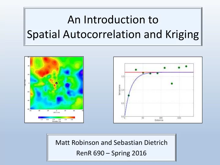

An Introduction to Spatial Autocorrelation and Kriging Matt Robinson and Sebastian Dietrich RenR 690 – Spring 2016
Tobler and Spatial Relationships • Tobler’s 1 st Law of Geography : “Everything is related to everything else, but near things are more related than distant things.” 1 • Simple but powerful concept • Patterns exist across space • Forms basic foundation for concepts related to spatial dependency Waldo R. Tobler (1) Tobler W., (1970) "A computer movie simulating urban growth in the Detroit region". Economic Geography , 46(2): 234-240.
Spatial Autocorrelation (SAC) – What is it? • Autocorrelation : A variable is correlated with itself (literally!) • Spatial Autocorrelation : Values of a random variable, at paired points, are more or less similar as a function of the distance between them 2 Closer Points more similar = Positive Autocorrelation Closer Points less similar = Negative Autocorrelation (2) Legendre P. Spatial Autocorrelation: Trouble or New Paradigm? Ecology. 1993 Sep;74(6):1659 – 1673.
What causes Spatial Autocorrelation? (1) Artifact of Experimental Design (sample sites not random) Parent Plant (2) Interaction of variables across space (see below) Univariate case – response variable is correlated with itself Eg. Plant abundance higher (clustered) close to other plants (seeds fall and germinate close to parent). Multivariate case – interactions of response and predictor variables due to inherent properties of the variables Eg. Location of seed germination function of wind and preferred soil conditions Mechanisms underlying patterns will depend on study system!!
Why is it important? Presence of SAC can be good or bad (depends on your objectives) Good : If SAC exists, it may allow reliable estimation at nearby, non-sampled sites ( interpolation ). Bad : If SAC exists, observations are not independent (violates assumption of many statistical tests) Failure to recognize/account for SAC can lead to erroneous statistical results and conclusions
Structure Functions Spatial structure = spatial patterns in your data Structure Functions - mathematical functions that describe spatial autocorrelation and spatial structure 3 Include terms that account for distance between sites Most common structure functions based on variance (variogram) and covariance ( correlogram ) (3) Legendre P, Fortin MJ. 1989. Spatial pattern and ecological analysis. Vegetation . 80(2):107 – 138.
Tests for SAC: Moran’s I Moran’s I (Moran’s Index): Measures degree of correlation between sample/observation points based on both variable values and distance between points 4 Determines whether spatial pattern in data is random , clustered , or dispersed. (4) How Spatial Autocorrelation (Global Moran’s I) works - (ArcGIS Desktop Help). Available from: http://help.arcgis.com/En/Arcgisdesktop/10.0/Help/index.html#//005p0000000t000000
Moran’s I - Explained Extension of Pearson’s Correlation Coefficient , r Pearson’s (r): Measures association between 2 different variables Moran’s I : Measures degree of association of single variable with itself at different points in space as a function of distance between points (called a spatial lag ) 5 Range: -1.0 (negative SAC) and 1.0 (positive SAC) Value close to zero indicates no/little SAC (5) Fortin, M.J., Dale, M.R. and Ver Hoef, J.M. 2002. Spatial analysis in ecology. Encyclopedia of environment.
Math Behind Moran’s I (1) Calculate Matrix of Inverse Distance Weights - Distance weight Variable x at defines spatial relationship between all sample (from matrix) points i and j point pairs within a specified area. Observed I S 0 = Sum of all weights (2) Calculate Observed and Expected Moran I Expected I (Under H 0 of No SAC) (3) Compare to Observed to Expected Moran’s I (expected under H 0 of no SAC)
Moran’s I: In R (using package “ape”) (1) Input dataframe Response variable x and y coordinates (specify location of sample points to be tested) Example Dataframe Station Av8top Lat Lon 1 60 7.225806 34.13583 -117.9236 2 69 5.899194 34.17611 -118.3153 (3) Run Moran’s I Function 3 72 4.052885 33.82361 -118.1875 4 74 7.181452 34.19944 -118.5347 Moran.I(ozone$Av8top, ozone.dists.inv) 5 …….. (2) Calculate Inverse Distance Matrix zone.dists <- as.matrix(dist(cbind(ozone$Lon, ozone$Lat))) ozone.dists.inv <- 1/ozone.dists diag(ozone.dists.inv) <- 0 ozone.dists.inv[1:5, 1:5] Source: http://www.ats.ucla.edu/stat/r/faq/morans_i.htm
Moran’s I: Output and Interpretation In R Moran’s I is an Inferential Statistic - Must examine in Context of Null Hypothesis (No Spatial Autocorrelation) Observed > Expected : values cluster spatially (1) Look at p-value ( + autocorrelation) Significant p-value: reject H 0 (Autocorrelation exists). Observed < Expected values disperse spatially (2) Examine Observed and Expected Moran’s I (- autocorrelation) Observed = Moran’s I calculated from the data Expected = Moran’s I expected under H 0 (no spatial autocorrelation) Output in R sd = standard deviation of Moran’s I under H 0 p.value = p-value of the test of H 0 against H A Source: http://www.ats.ucla.edu/stat/r/faq/morans_i.htm Source: http://www.inside-r.org/packages/cran/ape/docs/Moran.I
Other Autocorrelation Indices • Geary’s C – (similar to Moran’s) - more sensitive to differences in small spatial neighborhoods • Moran’s I – global measurement; sensitive to extreme Geary’s C values Result in similar conclusions, but Moran’s generally preferred (more powerful) 5,6 For more information see: http://geog.ucsb.edu/~chris/readings/Spatial.Analysis.in.Ecology.Encyclopedia.E nvironmetrics.pdf (5) Cliff, AD and Ord, JK (1975). The choice of a test for spatial autocorrelation. In J. C. Davies and M. J. McCullagh (eds) Display and Analysis of Spatial Data , John Wiley and Sons, London, 54-77 (6) Cliff, A. D. and Ord, J. K. 1981 Spatial processes - models and applications. (London: Pion).
The Variogram Georges François Paul Marie Matheron December 2, 1930 – August 7, 2000 French mathematician and geologist, known as the founder of geostatistics Georges Matheron Princ ncip iple les s of geostat atist istics ics Economic Geology 1963 58:1246-1266 Source: http://faculty.washington.edu/edford/Variogram.pdf
Variogram continued All credit to / Source: http://faculty.washington.edu/edford/Variogram.pdf The variogram in a more ecologic context: The experimental variogram allows the description of the overall spatial pattern and the estimation of spatial autocorrelation parameters: (a) the spatial range, a, where the variable is spatially influenced by the same underlying process; (b) the nugget effect, which is the estimate of the error inherent in the measurements (sampling design and sampling unit size) and environmental variability; and (c) the sill that quantifies the spatial pattern intensity Secondly we derive a theoretical variogram which can be used for prediction of values (kriging) All credit to / Source (good read!): Spatial analysis in ecology Marie-Josee Fortin, Mark R.T. Dale & Jay ver Hoef ´ Volume 4, pp 2051 – 2058 in Encyclopedia of Environmetrics http://geog.ucsb.edu/~chris/readings/Spatial.Analysis.in.Ecology.Encyclopedia.Environmetrics.pdf
Suggested read Variogram: Variogram or Semivariogram? Variance or Semivariance? Allan Variance or Introducing a New Term? Martin Bachmaier , Matthias Backes Mathematical Geosciences August 2011, Volume 43, Issue 6, pp 735-740 First online: 01 July 2011
The history of Kriging Some history: Method developed by Professor Daniel Gerhardus Krige The concept of Support is very basic to geostatistics and was first covered by Ross (1950) and further developed by Krige (1951), including Krige’s variance- size of area relationship. 37 Spatial Structure and Variograms The corresponding correlograms or covariograms were used on a Simple Kriging basis for block evaluations Initially Professor Krige’s regressed estimates were then still called ‘weighted moving averages’ until Matheron’s insistence in the mid- 1960 ’s on the term Kriging in recognition of Professor Krige’s pioneering work. Matheron, also then proposed the use of the variogram to define the spatial structure. This model is an extension and refinement of the concept covered by De Wijs (1951/3); (Source:https://www.goldfields.com/pdf/presentations/2015/summary_prof_danie_krige_m emorial_lecture.pdf) The theoretical basis for the method was developed by the French mathematician Georges Matheron based on the Master's thesis of Danie G. Krige , the pioneering plotter of distance-weighted average gold grades at the Witwatersrand reef complex in South Africa. (Source: https://en.wikipedia.org/wiki/Kriging)
Kriging – what it does • also known as BLUP (best linear unbiased prediction) • returning the observed values at sampling locations • interpolates values using the intensity and shape of the experimental and modeled variogram • using a neighborhood and/or distance search radius • provides the standard errors of the interpolated values All credit to / Source (good read!): Spatial analysis in ecology Marie-Josee Fortin, Mark R.T. Dale & Jay ver Hoef ´ Volume 4, pp 2051 – 2058 in Encyclopedia of Environmetrics http://geog.ucsb.edu/~chris/readings/Spatial.Analysis.in.Ecology.Encyclopedia.Environmetrics.pdf
Recommend
More recommend