AIXI: Universal Optimal Sequential Decision Making Marcus Hutter - PowerPoint PPT Presentation
AIXI: Universal Optimal Sequential Decision Making Marcus Hutter (2005) Reinforcement Learning State space , Action space , Policy , Reward (, ) Goal: Find policy which maximizes expected cumulative reward.
AIXI: Universal Optimal Sequential Decision Making Marcus Hutter (2005)
Reinforcement Learning • State space 𝑇, Action space 𝐵, Policy 𝜌, Reward 𝑆(𝑏, 𝑡) • Goal: Find policy which maximizes expected cumulative reward. • Challenge: Environment which RL interacts with is unknown • Explore and approximate the environment • Hard to balance exploration vs exploitation • AIXI: why approximate one environment? Consider them all!
Optimal Agents in Known Environments • , 𝒫, 𝑆 = ( action, observation, reward) spaces • 𝑏 - = action at time 𝑙 , 𝑦 - = 𝑝 - 𝑠 - = perception at time 𝑙 • Agent follows policy 𝜌: ×𝒫×ℛ ∗ → • Environment reacts with 𝜈: ×𝒫×ℛ ∗ × → 𝒫×ℛ
Agent-Environment Visualization
Optimal Agents in Known Environments • Performance of 𝜌 is expected cumulative reward A : = 𝔽 9 9: ] : [= 𝑊 𝑠 9 > >?@ • If 𝜈 is true environment, optimal policy is 𝑞 9 ≔ arg max : 𝑊 9 : ?
Definition of the Environment • An environment, 𝜍 , is a sequence of conditional probability functions {𝜍 L , 𝜍 @ , 𝜍 M , … } and is unknown to the agent • Each element in the sequence satisfies the “chronological condition” : ∀𝑏 @:Q ∀𝑦 @:QR@ : 𝜍 QR@ (𝑦 @:QR@ 𝑏 @:QR@ = = 𝜍 Q (𝑦 @:Q |𝑏 @:Q ) S T ∈V
Definition of the Environment ∀𝑏 @:Q ∀𝑦 @:QR@ : 𝜍 QR@ (𝑦 @:QR@ 𝑏 @:QR@ = = 𝜍 Q (𝑦 @:Q |𝑏 @:Q ) S T ∈V Conditioned Conditioned on all actions on all actions up to 𝑜 − 1 Marginalization of 𝜍 Q over up to 𝑜 the current observation- reward
Dealing with the Unknown Environment • The idea is to maintain a mixture of environment models, in which each model is assigned a weight that represents the agent’s confidence in what it believes is the true environment • As the agent obtains more experience, it updates the weights and thus its belief of the underlying environment • Reminiscent of a Bayesian agent
Mixture Model • ℳ ≜ {𝜍 @ , 𝜍 M , … , 𝜍 Q } is the countable class of environments ^ > 0 is the weight assigned to each 𝜍 ∈ ℳ such that ∑ ^∈ℳ 𝑥 L ^ = • 𝑥 L 1 ^ 𝜍(𝑦 @:Q |𝑏 @:Q ) 𝜊 𝑦 @:Q |𝑏 @:Q ≜ = 𝑥 L ^∈ℳ
Selecting a Universal Prior • Occam’s Razor: The simplest solution is the most likely ^ = 1 • Formalized as Kolmogorov Complexity ∑ ^∈ℳ 𝑥 L Type equation here. ^ 𝜍(𝑦 @:Q |𝑏 @:Q ) 𝜊 𝑦 @:Q |𝑏 @:Q ≜ = 𝑥 L ^∈ℳ “Yo.”
Kolmogorov Complexity • Length of the shortest program on a Universal Turing Machine which specifies an object • In our domain: shortest program which produces environment 𝜍 𝐿 𝜍 ≔ min 𝑚𝑓𝑜𝑢ℎ 𝑞 : 𝑉 𝑞 = 𝜍 p • Advantage: completely independent of prior assumptions • Problem: Incomputable due to halting problem. • Naïve search over all inputs will contain those with infinite loops • Paradoxical: “Shortest object describable by N bits” is less than N bits.
Solomonoff Prior • Key idea: Use inverse Kolmogorov Complexity as environmental prior to compute mixture over all possible environments 2 Rz(^) ∗ 𝑊 : Υ 𝜌 = = ^ ^∈ℳ x • Υ 𝜌 measures agent’s ability to perform in all possible environments • Hutter describes this Υ 𝜌 as Universal Intelligence
AIXI • Expectimax over Solomonoff Prior • ℳ are chronologically conditional environments • Converges to agent acting with knowledge of true environment • Mathematically proven
Evaluation: Pros and Cons • Theoretically optimal decision making. • Proven to converge to optimal agent acting in true environment • Universal • Prior completely independent of actual environment behavior • “Reduces any conceptual AI problem to computation problem” • Incomputable and Intractable • Cannot compute Kolgomorov Complexity • Reward function? • Unclear how to define reward function which is also independent of problem
Related Works: Approximations • Work in AIXI mainly in approximating the theoretical framework. • AIXI 𝑢𝑚 • Marcus Hutter. Universal algorithmic intelligence: A mathematical top→down approach. In B. Goertzel and C. Pennachin, editors, Artificial General Intelligence, Cognitive Technologies, pages 227–290. Springer, Berlin, 2007. ISBN 3-540-23733-X. URL http://www.hutter1.net/ai/aixigentle.htm. • Summary: provides approximate AIXI which is more optimal than any other RL agent with the same time and space constraints. • MC-AIXI (Next!) • Summary: Monte Carlo approximation of AIXI.
MC-AIXI CTW • “Monte Carlo – AIXI with Context Tree Weightings” • Veness et al 2011 • Solves main barriers to applying AIXI: 1. Expectimax is intractable → Estimate using MCTS 2. Kolmogorov Complexity is incomputable → Replace universe of environments with smaller model class with surrogate for complexity
Part 1: MCTS • 𝜍 UCT is used to estimate AIXI Expectimax by adapting the classic selection-expansion-rollout-backprop MCTS algorithm • Decision node (circle): • Contains a history, h , and a value function estimate, { 𝑊(ℎ) • It has children (called “Chance nodes”) corresponding to the number of possible actions • An action, a, is selected based on the UCB action-selection policy that balances exploration and exploitation • Chance node (star): • Follows a decision node • Contains the history, ha; an estimate of the future value, { 𝑊(ℎ𝑏) ; and the environment model, 𝜍(⋅ |ℎ𝑏) , that returns a percept conditioned on the history • A new child of the chance node is added when a new percept is received
Part 2: Approximating the Solomonoff Prior • Solomonoff Prior: ∑ ^ 2 Rz(^) is incomputable • Solution: Replace with smaller class of environments • Variable Order Markov Process • Calculates probability of next observation depending on last k observations • Replace entire universe of environments with mixture of Markov Processes
Prediction Suffix Tree • Representation of a sequence of binary events • Able to encode all variable order Markov Models up to depth D • Represents a space of 2^2^D
Context Tree Weighting • Provides method to evaluate PST in linear time • Naively computable in 𝒫 (2^2^D), CTW algorithm reduces to 𝒫 (D) • Smaller trees represent simpler Markov Models • Evaluate prior probability under Occam’s razor as size of tree Γ ~ 𝑁 = # nodes in PST • Replace Kolmogorov prior with CTW prior
Context Tree Weighting: Updated Formula • Original intractable prior • MC-AIXI with CTW
Algorithm Performance Partially Observable Pacman Cheese Maze • The agent must navigate to a piece of cheese • -1 for entering an open cell Agent is unaware of the monsters’ • • -10 for hitting a wall locations and the maze • +10 for finding cheese It can only “smell” food and observe • food in its direct line of sight
Performance on Cheese Maze
Performance on PO-Pacman
Related Work • Andrew Kachites McCallum. Reinforcement Learning with Selective Perception and Hidden State . PhD thesis, University of Rochester, 1996 ⟶ "𝑉𝑢𝑗𝑚𝑗𝑢𝑧 𝑇𝑣𝑔𝑔𝑗𝑦 𝑁𝑓𝑛𝑝𝑠𝑧“ • V.F. Farias, C.C.Moallemi, B. Van Roy, and T.Weissman. Universal reinforcement learning. Information Theory, IEEE Transactions on , 56(5):2441 –2454, may 2010. ⟶ "𝐵𝑑𝑢𝑗𝑤𝑓 − 𝑀𝑎"
Timeline Context Tree MCTS Weightings MC-AIXI-CTW “Bandit based MC Solomonoff Induction Planning” Willems, Shtarkov, Veness et al Kocsis & Szepesvari Ray Solomonoff Tjalkens 2010 2006 1960’s 1995 Kolmogorov Complexity AIXI AIXI 𝑢𝑚 Marcus Hutter Andrey Kolmogorov 2005 Marcus Hutter 1963 2007
MC-AIXI-CTW Playing Pac-Man • jveness.info/publications/pacman_jair_2010.wmv
Recommend
More recommend
Explore More Topics
Stay informed with curated content and fresh updates.
