AIRS CO2 assimilation with an EnKF: preliminary results Junjie Liu , - PowerPoint PPT Presentation
AIRS CO2 assimilation with an EnKF: preliminary results Junjie Liu , Eugenia Kalnay, Inez Fung, Moustafa T. Chahine, Edward T. Olsen NASA Sounder Science Team Meeting Oct. 15, 2009 0 Motivation & Outline Motivation: To estimate CO2
AIRS CO2 assimilation with an EnKF: preliminary results Junjie Liu , Eugenia Kalnay, Inez Fung, Moustafa T. Chahine, Edward T. Olsen NASA Sounder Science Team Meeting Oct. 15, 2009 0
Motivation & Outline Motivation: • To estimate CO2 vertical profile based on AIRS CO2 retrievals, and explore deriving surface carbon fluxes. Outline: • AIRS CO2 comparison with model simulation for year 2003: CAM3.5 does not do so well • AIRS CO2 assimilation method and results • Comparisons between assimilation runs with and without assimilating CO2 • Discussion, challenges and plans. 1
CO 2 simulation in CAM3.5 • Community Atmospheric Model 3.5 (CAM 3.5) coupled with Community Land Model 3.5 (CLM 3.5) – Finite Volume dynamical core – 2.5°x1.9° horizontal resolution, with 26 vertical levels up to 3.5hPa. • CO 2 is transported as a tracer in CAM 3.5 • Carbon surface fluxes: – Fossil fuel emission (yearly average value for 2003) – Ocean C fluxes (monthly means, interpolated between months; Takahashi et al., 2002) – Land C flux (6-hourly carbon flux from CASA) • Initial CO2 is the spin-up after 3 years. • CO2 from this model run is the “ nature run ”. 2
Comparison between AIRS CO2 & model simulation: annual mean Unit: ppm AIRS CO2 annual mean in 2003 Nature CO2 = Model CO2 - offset Offset= annual mean model CO2 - annual mean AIRS CO2 ~1ppm Nature CO2 annual mean in 2003 Nature run has rather different spatial patterns than the AIRS CO2 annual mean; Likely due to the vertical mixing in the model. 3
Comparison between AIRS CO2 & model simulation (convolved with AIRS aver. kernel) Unit: ppm AIRS CO2 annual mean in 2003 Nature CO2 = Model CO2 - offset Offset= annual mean model CO2 - annual mean AIRS CO2 Nature CO2 annual mean in 2003 Nature run has rather different spatial patterns than the AIRS CO2 annual mean; Likely due to not enough vertical mixing in the model. 4
AIRS comparison with model simulation Surface CO2 North-South gradient Unit: ppm Model simulation N-S gradient from model simulation is similar but larger than surface CO2 observations. surface observation Difference between AIRS and model simulation N-S gradient from model is smaller than AIRS CO2: • Inaccuracies in vertical mixing in the model; • Inaccurate boundary flux forcing. 5
Seasonal cycle: model and AIRS 20ºN-60ºN 20ºS-20ºN AIRS CO2 MODEL CO2 MODEL CO2 AIRS CO2 60ºS-20ºS AIRS CO2 In the NH the seasonal cycle is similar but weaker in the model than AIRS. MODEL CO2 No significant seasonal cycle in the tropics in the AIRS data. Units: ppm 6
Seasonal cycle: model and AIRS 20ºN-60ºN 20ºS-20ºN AIRS CO2 MODEL CO2 MODEL CO2 AIRS CO2 Surface 60ºS-20ºS Max CO2 AIRS CO2 In the NH the seasonal cycle is similar but weaker in the model than AIRS. MODEL CO2 AIRS CO2 max delayed about a month wrt to surface max, model delayed another month: vertical mixing? Units: ppm 7
CO 2 assimilation with EnKF • Model forecast x b is a CO 2 vertical profile; • AIRS CO 2 is weighted column Volume Mixing Ratio (vmr); => observation operator: interpolate x b to obs location & convolve the CO2 vertical profile with averaging kernel A(x, y, t). k y b = h ( x b ) = A T ( Hx b ) = � b ) a i ( Hx i i = 1 x b : model forecast CO 2 vertical profile; k: number of vertical levels; H: spatial interpolation operator; y b : model predicted CO 2 column mixing ratio. A : averaging kernel; a i is the element at ith vertical level; 8
CO 2 assimilation method • AIRS CO 2 observation is a column weighted value; • Model forecast CO 2 state x b and analysis state x a are vertical profiles; => How to localize CO 2 column observation to obtain CO 2 vertical profile? o � = a i � ( y o � h ( x b )); localize the column observation increment to i th � y i vertical level by the ith averaging kernel element a i So far we have assimilated the CO2 independently of the other variables, in a univariate approach. Multivariate assimilation, like we have done with moisture retrievals, may be better, but it is more subject to sampling errors in the covariance between CO2 and the transporting wind. 9
Analysis increment and observation increment at one analysis time Observation increment (shaded) & Observation increment: column analysis increment (contour) observation minus 6-hour forecast; (blue: negative; red: positive) Analysis increment: analysis mean minus background mean integrated over the column; (dashed: negative; solid: positive) The correction to the forecast is consistent with the difference between the observation and the background. 10
Analysis increment & observation increment at one analysis time Observation increment (shaded) & Observation increment: column analysis increment (contour) observation minus 6-hour forecast; (blue: negative; red: positive) Analysis increment: analysis mean minus background mean integrated over the column; (dashed: negative; solid: positive) What is the vertical profile of analysis increment? Cut through the black line to get vertical analysis increment profile. 11
Analysis increment vertical profile & averaging kernel vertical profile The correction to the forecast spans from middle to upper troposphere. consistent with the span of the average averaging kernel. 12
Comparison of two assimilation runs, with and without AIRS CO2 Meteo run AIRS run CAM3.5+CLM3.5 CAM3.5+CLM3.5 (u, v, T, Ps) (u, v, T, Ps) analysis analysis (CO 2 ) analysis 6 hour forecast 6 hour forecast (u, v, T, q, Ps) (CO 2 ) (u, v, T, q, Ps) (CO 2 ) LETKF LETKF LETKF Observations AIRS CO 2 Observations (u,v,T,q,Ps) (u,v,T,q,Ps) • In Meteo run we assimilate u,v,T,q,Ps: no constraints on model CO 2 . • In AIRS run we also assimilate AIRS CO2. • We run two months of assimilation for both experiments. 13
Monthly mean spatial anomaly CO2 in Jan. AIRS CO2 CO2 from AIRS run CO2 from Meteo run Plotted value =ave(CO2) time - ave(ave(CO2) time ) space 14
Monthly mean spatial anomaly CO2 in Jan. AIRS CO2 CO2 from AIRS run CO2 from Meteo run Plotted value =ave(CO2) time - ave(ave(CO2) time ) space The spatial pattern from the AIRS run is closer to the AIRS CO2 observations 15
Monthly mean spatial anomaly CO2 in Feb. AIRS CO2 CO2 from AIRS run CO2 from meteo run Plotted value =ave(CO2) time - ave(ave(CO2) time ) space The spatial pattern from the AIRS run is closer to the AIRS CO2 observations: also closer in February than in January. 16
Monthly mean spatial anomaly CO2 between mid-Feb and mid-Mar CO2 from AIRS run AIRS CO2 CO2 from meteo run Plotted value =ave(CO2) time - ave(ave(CO2) time ) space The spatial pattern is further improved. 17
AIRS run (top), convolved CO2 from AIRS CO2 (bottom), averaged over three assimilation cycles (a “snapshot” comparison) 18ZJan09-12ZJan10 18ZMarch16-12ZMarch17 18
Propagation of CO2 information vertically 25S-25N 25N-70N 60S-25S Zonal average of the difference in ? CO2 from AIRS run and from Meteo run The difference between AIRS run CO2 and Meteo run CO2 propagates the peak of the averaging kernel (200hPa-400hPa) downward from with time. AIRS CO2 may provide some info on surface CO2 fluxes. 19
Conclusions and Discussion • Annual mean CO2 from model simulation has different spatial patterns from AIRS CO2, and a delayed maximum. • This may be due to inaccurate surface carbon flux forcing and the inaccurate vertical mixing in the model. • Assimilation of AIRS CO2 corrects the model simulation results, not only in a single level but in the whole vertical profile through the averaging kernel. • Propagated by both assimilation and model transport, the AIRS CO2 information propagates to the surface, which may help to infer surface carbon fluxes. • The inflation of the error covariance needs to be improved. 20
Challenges and Future work • Time lag between AIRS CO2 and local carbon flux: – AIRS CO2 may include carbon flux information upstream due to air transport: we will try multivariate assimilation (but this introduces further sampling errors). Inflation needs work. • Longer spin-up time for CO2 than for meteorological variables. – Only one piece information to correct a vertical profile. • EnKF is good at estimating parameters. Can we use of AIRS CO2 to estimate vertical mixing parameters? • Include the offset (bias) between nature run and AIRS CO2 in the assimilation. • Assimilate the CO2 observations for the whole year of 2003. • Compare the results to in-situ CO 2 observations, e.g., aircraft data. • The simulation EnKF experiments of Ji-Sun Kang (UMD) suggest that it is possible to estimate surface carbon fluxes based on AIRS CO 2 and GOSAT CO 2 data if the model biases are accounted for. 21
Recommend
More recommend
Explore More Topics
Stay informed with curated content and fresh updates.
