AIRS CO 2 data assimilation with Ensemble Kalman filter: preliminary - PowerPoint PPT Presentation
AIRS CO 2 data assimilation with Ensemble Kalman filter: preliminary results Junjie Liu 1 Eugenia Kalnay 2 and Inez Fung 1 1 UC Berkeley; 2 University of Maryland Many thanks to Edward Olsen and Moustafa Chahine for kindly providing us their AIRS
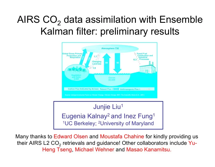
AIRS CO 2 data assimilation with Ensemble Kalman filter: preliminary results Junjie Liu 1 Eugenia Kalnay 2 and Inez Fung 1 1 UC Berkeley; 2 University of Maryland Many thanks to Edward Olsen and Moustafa Chahine for kindly providing us their AIRS L2 CO 2 retrievals and guidance! Other collaborators include Yu- Heng Tseng, Michael Wehner and Masao Kanamitsu.
AIRS CO 2 data assimilation with Ensemble Kalman filter: preliminary results Junjie Liu 1 Inez Fung 1 and Eugenia Kalnay 2 1 UC Berkeley; 2 University of Maryland Many thanks to Edward Olsen and Moustafa Chahine for kindly providing us their AIRS L2 CO 2 retrievals and guidance! Other collaborators include Yu- Heng Tseng, Michael Wehner and Masao Kanamitsu.
Motivation & Goals Motivation: Accurate carbon flux estimation from inversion needs far more CO 2 observations than current surface obs can provide . Goals: AIRS CO2 at 18Z01May2003 (+/-3hour) 1. Generate global CO 2 map every 6- hour; start with AIRS, then GoSat 2. Propagate AIRS CO 2 in both horizontal and vertical direction through data assimilation and transport model
Outline • CO 2 simulation in Community Atmospheric Model 3.5 (CAM 3.5) • Methods to assimilate AIRS CO 2 with Ensemble Kalman Filter (EnKF) • Preliminary results • Summary and future plans
CO 2 simulation in CAM3.5 • Community Atmospheric Model 3.5 (CAM 3.5) coupled with Community Land Model 3.5 (CLM 3.5) – Finite Volume dynamical core – 2.5°x1.9° horizontal resolution, with 26 vertical levels up to 3.5hPa. • CO 2 is transported as a tracer in CAM 3.5 • Carbon flux forcing – Fossil fuel emission (yearly average value in 2003) – Ocean C flux (changes with month; Takahashi et al., 2002) – Land C flux (changes with month; CASA annually balanced flux from Transcom 3) • Four-year model integration started from 01Jan 2000
Comparison between model simulation and observations CO 2 seasonal cycle mean north-south CO 2 gradient Model: black ; Model: solid ; obs:green obs: dashed line; red: year 2002; black: year 2003. • Seasonal cycle simulation is pretty good even though the flux is not perfect. • N-S model gradient is smaller than observations, similar to Engelen at al. 2008.
Ensemble Kalman Filter Observation y o & its uncertainty Analysis ensemble & its uncertainty Background ensemble x b & its uncertainty t0 t1 t2 x a = x b + K ( y o � h ( x b )), K is function of background Analysis mean error and observation error. h ( � ) is the observation operator, which interpolates model forecast to observation space (more details later);
CO 2 observation operator • Model forecast x b is CO 2 vertical profile; • AIRS CO 2 is weighted column Volume Mixing Ratio (vmr); => observation operator: interpolate x b to obs location & calculate model forecast weighted column CO 2 vmr based on CO 2 profile. k y b = h ( x b ) = A T ( Hx b ) = � b ) a i ( Hx i i = 1 x b : model forecast CO 2 vertical profile; k: the total vertical levels; H: spatial interpolation operator; y b : model predicted CO 2 column mixing ratio. A : averaging kernel; a i is the element at ith vertical level;
Averaging Kernel Averaging kernel for 390ppm Averaging kernel for 370ppm (black: 90º; red: 45º; green: 0º) (black: 90º; red: 45º; green: 0º) 1. Interpolate averaging kernels based on CO 2(base) CO2(base)(time=t)=371.92429+1.840618*(t-t0), where t0=00ZJan1, 2002; 2. Linearly Interpolate among latitudes ; 3. Normalize the interpolated averaging kernels, i.e., sum(A)=1.0
CO 2 assimilation method • AIRS CO 2 observation is a column weighted value; • Model forecast CO 2 state x b and analysis state x a are vertical profiles; => How to localize CO 2 column observation to obtain CO 2 vertical profile? o � = a i � ( y o � h ( x b )); localize the column observation increment to i th � y i vertical level by the ith averaging kernel element a i b � = a i � h ( x j b ); localize the j th ensemble forecast column CO 2 to the i th � y j , i vertical level by the i th averaging kernel element a i
AIRS CO 2 observations 00Z02May, 2003 +-3hour • Some outliers in the AIRS CO2 observations (may not mean bad quality). • Need some quality control before assimilating these obs.
Quality control of AIRS CO2 observations 00Z02May, 2003 +-3hour Before buddy check After buddy check Buddy check: compare each observation to the mean of the observations within 400km. Bad observations : absolute difference larger than 5ppm; filter out about 8%.
Single CO 2 analysis step 350 hPa CO 2 analysis increment (ppm) CO 2 at 00Z01May2003 (+3hour) after QC • Analysis increment= analysis-background forecast • Spatial pattern of analysis increment follows the observation coverage. • Propagate observation information horizontally.
CO 2 analysis increment vertical profile Along 5ºw • The magnitude of analysis increments in vertical direction follows the shape of averaging kernel.
Experimental design Meteorological run CO 2 run CAM3.5+CLM3.5 CAM3.5+CLM3.5 (u, v, T, Ps) (u, v, T, Ps) analysis analysis (CO 2 ) analysis 6 hour forecast 6 hour forecast (u, v, T, q, Ps) (CO 2 ) (u, v, T, q, Ps) (CO 2 ) LETKF LETKF LETKF Observations AIRS CO 2 Observations (u,v,T,q,Ps) (u,v,T,q,Ps) • No constraints on CO 2 in meteorological run; • AIRS CO 2 constrains CO 2 vertical profile in CO 2 run.
CO 2 difference between CO 2 run and meteorological run Unit: ppm 1. Adjustment by AIRS CO 2 spans from 800hPa to 100hPa 2. The adjustment is larger in the NH
Fitting to AIRS CO 2 obs Green: meteorological run; Red: 6-hour forecast from CO 2 run; black: analysis from CO 2 run NH SH Fitting to the AIRS CO 2 observations has been much improved in CO 2 run.
Summary • CO 2 seasonal cycle is well simulated by CAM3.5, but N-S gradient is weaker; • Proposed a procedure to assimilate AIRS CO 2 retrievals with ensemble Kalman filter; • Assimilation and transport model propagate the AIRS CO 2 observation in both horizontal and vertical directions. • As expected, CO 2 column mixing ratio from CO 2 run is closer to AIRS CO 2 retrievals than that from meteorological run.
Future plans • Extend the length of assimilation and use more accurate averaging kernel. • Compare the results to in-situ CO 2 observations, e.g., aircraft data. • Develop more sophisticated QC. • Explore multivariate CO 2 data assimilation. • Use carbon flux predicted by the online CASA model. • Based on the simulated experiments of Ji-Sun Kang (UMD), ultimately, estimate carbon flux based on AIRS CO 2 data and GOSAT CO 2 data
Recommend
More recommend
Explore More Topics
Stay informed with curated content and fresh updates.
