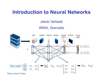
Advanced Learning Models Julien Mairal and Jakob Verbeek Inria - PowerPoint PPT Presentation
Advanced Learning Models Julien Mairal and Jakob Verbeek Inria Grenoble MSIAM/MoSIG, 2018/2019/ Julien Mairal Advanced Learning Models 1/16 Goal Introducing two major paradigms in machine learning called kernel methods and neural networks.
Advanced Learning Models Julien Mairal and Jakob Verbeek Inria Grenoble MSIAM/MoSIG, 2018/2019/ Julien Mairal Advanced Learning Models 1/16
Goal Introducing two major paradigms in machine learning called kernel methods and neural networks. Ressources check the website of the course. http://thoth.inrialpes.fr/ people/mairal/teaching/2018-2019/MSIAM/ . Grading 1 homework (30%), one data challenge (30%) and one exam (40%). 1 data challenge; can also be done by teams of two students; Julien Mairal Advanced Learning Models 2/16
Common paradigm: optimization for machine learning Optimization is central to machine learning. For instance, in supervised learning, the goal is to learn a prediction function f : X → Y given labeled training data ( x i , y i ) i =1 ,...,n with x i in X , and y i in Y : n 1 � min L ( y i , f ( x i )) + λ Ω( f ) . n f ∈F � �� � i =1 regularization � �� � empirical risk, data fit [Vapnik, 1995, Bottou, Curtis, and Nocedal, 2016]... Julien Mairal Advanced Learning Models 3/16
Common paradigm: optimization for machine learning Optimization is central to machine learning. For instance, in supervised learning, the goal is to learn a prediction function f : X → Y given labeled training data ( x i , y i ) i =1 ,...,n with x i in X , and y i in Y : n 1 � min L ( y i , f ( x i )) + λ Ω( f ) . n f ∈F � �� � i =1 regularization � �� � empirical risk, data fit The scalars y i are in {− 1 , +1 } for binary classification problems. { 1 , . . . , K } for multi-class classification problems. R for regression problems. R k for multivariate regression problems. Julien Mairal Advanced Learning Models 3/16
Common paradigm: optimization for machine learning Optimization is central to machine learning. For instance, in supervised learning, the goal is to learn a prediction function f : X → Y given labeled training data ( x i , y i ) i =1 ,...,n with x i in X , and y i in Y : n 1 � min L ( y i , f ( x i )) + λ Ω( f ) . n f ∈F � �� � i =1 regularization � �� � empirical risk, data fit Example with linear models: logistic regression, SVMs, etc. assume there exists a linear relation between y and features x in R p . f ( x ) = w ⊤ x + b is parametrized by w, b in R p +1 ; L is often a convex loss function; Ω( f ) is often the squared ℓ 2 -norm � w � 2 . Julien Mairal Advanced Learning Models 3/16
Common paradigm: optimization for machine learning A few examples of linear models with no bias b : n 1 1 � 2( y i − w ⊤ x i ) 2 + λ � w � 2 Ridge regression: min 2 . n w ∈ R p i =1 n 1 � max(0 , 1 − y i w ⊤ x i ) + λ � w � 2 Linear SVM: min 2 . n w ∈ R p i =1 n 1 � � � 1 + e − y i w ⊤ x i + λ � w � 2 Logistic regression: min log 2 . n w ∈ R p i =1 Julien Mairal Advanced Learning Models 4/16
Common paradigm: optimization for machine learning The previous formulation is called empirical risk minimization ; it follows a classical scientific paradigm: 1 observe the world (gather data); 2 propose models of the world (design and learn); 3 test on new data (estimate the generalization error). Julien Mairal Advanced Learning Models 5/16
Common paradigm: optimization for machine learning The previous formulation is called empirical risk minimization ; it follows a classical scientific paradigm: 1 observe the world (gather data); 2 propose models of the world (design and learn); 3 test on new data (estimate the generalization error). A general principle It underlies many paradigms: deep neural networks, kernel methods, sparse estimation. Julien Mairal Advanced Learning Models 5/16
Common paradigm: optimization for machine learning The previous formulation is called empirical risk minimization ; it follows a classical scientific paradigm: 1 observe the world (gather data); 2 propose models of the world (design and learn); 3 test on new data (estimate the generalization error). Even with simple linear models, it leads to challenging problems in optimization: develop algorithms that scale both in the problem size n and dimension p ; are able to exploit the problem structure (sum, composite); come with convergence and numerical stability guarantees; come with statistical guarantees . Julien Mairal Advanced Learning Models 5/16
Common paradigm: optimization for machine learning The previous formulation is called empirical risk minimization ; it follows a classical scientific paradigm: 1 observe the world (gather data); 2 propose models of the world (design and learn); 3 test on new data (estimate the generalization error). It is not limited to supervised learning n 1 � min L ( f ( x i )) + λ Ω( f ) . n f ∈F i =1 L is not a classification loss any more; K-means, PCA, EM with mixture of Gaussian, matrix factorization,... can be expressed that way. Julien Mairal Advanced Learning Models 5/16
Paradigm 1: Deep neural networks n 1 � min L ( y i , f ( x i )) + λ Ω( f ) . n f ∈F � �� � i =1 regularization � �� � empirical risk, data fit The “deep learning” space F is parametrized: f ( x ) = σ k ( A k σ k – 1 ( A k – 1 . . . σ 2 ( A 2 σ 1 ( A 1 x )) . . . )) . Finding the optimal A 1 , A 2 , . . . , A k yields an (intractable) non-convex optimization problem in huge dimension. Linear operations are either unconstrained (fully connected) or involve parameter sharing (e.g., convolutions). Julien Mairal Advanced Learning Models 6/16
Paradigm 1: Deep neural networks A quick zoom on convolutional neural networks What are the main features of CNNs? they capture compositional and multiscale structures in images; they provide some invariance ; they model local stationarity of images at several scales. state-of-the-art in many fields. [LeCun et al., 1989, 1998, Ciresan et al., 2012, Krizhevsky et al., 2012]... Julien Mairal Advanced Learning Models 7/16
Paradigm 1: Deep neural networks A quick zoom on convolutional neural networks What are the main open problems? very little theoretical understanding ; they require large amounts of labeled data ; they require manual design and parameter tuning ; how to regularize is unclear; [LeCun et al., 1989, 1998, Ciresan et al., 2012, Krizhevsky et al., 2012]... Julien Mairal Advanced Learning Models 7/16
Paradigm 1: Deep neural networks A quick zoom on convolutional neural networks How to use them? they are the focus of a huge academic and industrial effort ; there is efficient and well-documented open-source software ; [LeCun et al., 1989, 1998, Ciresan et al., 2012, Krizhevsky et al., 2012]... Julien Mairal Advanced Learning Models 7/16
Paradigm 2: Kernel methods n 1 � L ( y i , f ( x i )) + λ � f � 2 min H . n f ∈H i =1 map data x in X to a Hilbert space and work with linear forms : ϕ : X → H and f ( x ) = � ϕ ( x ) , f � H . φ F X [Shawe-Taylor and Cristianini, 2004, Sch¨ olkopf and Smola, 2002]... Julien Mairal Advanced Learning Models 8/16
Paradigm 2: Kernel methods n 1 � L ( y i , f ( x i )) + λ � f � 2 min H . n f ∈H i =1 First purpose: embed data in a vectorial space where many geometrical operations exist (angle computation, projection on linear subspaces, definition of barycenters....). one may learn potentially rich infinite-dimensional models . regularization is natural (see next...) Julien Mairal Advanced Learning Models 9/16
Paradigm 2: Kernel methods n 1 � L ( y i , f ( x i )) + λ � f � 2 min H . n f ∈H i =1 First purpose: embed data in a vectorial space where many geometrical operations exist (angle computation, projection on linear subspaces, definition of barycenters....). one may learn potentially rich infinite-dimensional models . regularization is natural (see next...) The principle is generic and does not assume anything about the nature of the set X (vectors, sets, graphs, sequences). Julien Mairal Advanced Learning Models 9/16
Paradigm 2: Kernel methods Second purpose: unhappy with the current Euclidean structure? lift data to a higher-dimensional space with nicer properties (e.g., linear separability, clustering structure). then, the linear form f ( x ) = � ϕ ( x ) , f � H in H may correspond to a non-linear model in X . x1 2 x1 x2 R 2 x2 Julien Mairal Advanced Learning Models 10/16
Paradigm 2: Kernel methods How does it work? representation by pairwise comparisons Define a “comparison function”: K : X × X �→ R . Represent a set of n data points S = { x 1 , . . . , x n } by the n × n matrix : K ij := K ( x i , x j ) . X φ (S)=(aatcgagtcac,atggacgtct,tgcactact) S 1 0.5 0.3 K= 0.5 1 0.6 0.3 0.6 1 Julien Mairal Advanced Learning Models 11/16
Paradigm 2: Kernel methods Theorem (Aronszajn, 1950) K : X × X → R is a positive definite kernel if and only if there exists a Hilbert space H and a mapping ϕ : X → H , such that for any x, x ′ in X , K ( x, x ′ ) = � ϕ ( x ) , ϕ ( x ′ ) � H . φ F X Julien Mairal Advanced Learning Models 12/16
Recommend
More recommend
Explore More Topics
Stay informed with curated content and fresh updates.
