Adaptive Polygonization of Implicit Surfaces Ulises - PDF document

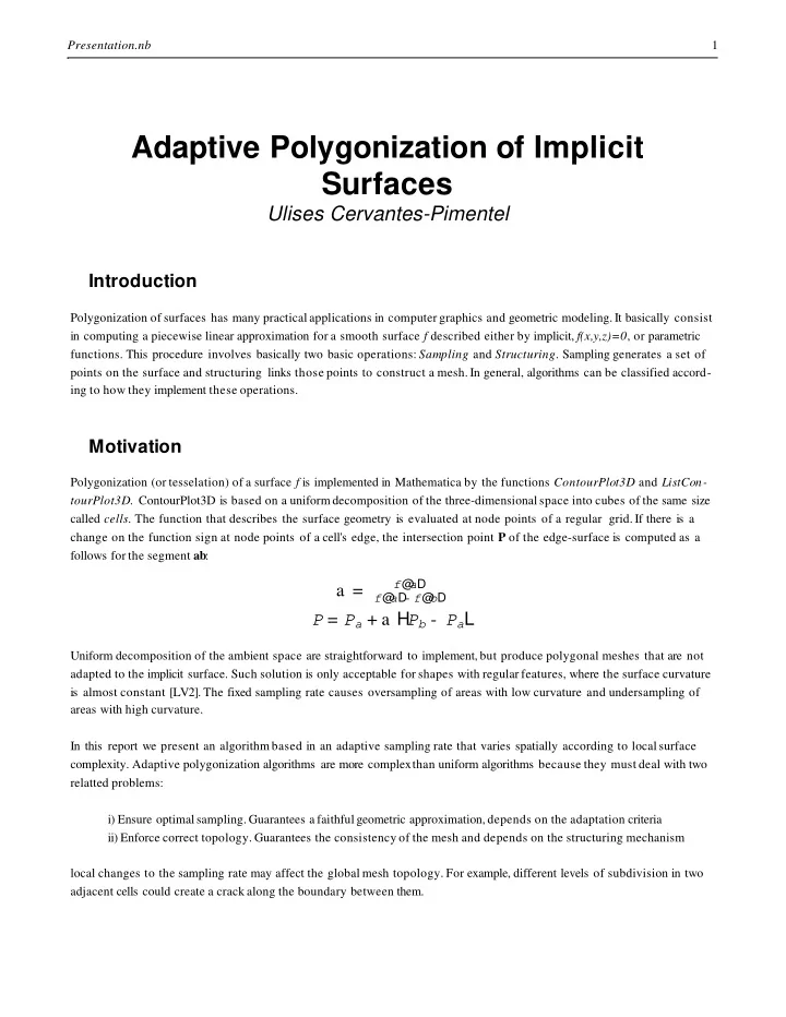
Presentation.nb 1 Adaptive Polygonization of Implicit Surfaces Ulises Cervantes-Pimentel � Introduction Polygonization of surfaces has many practical applications in computer graphics and geometric modeling. It basically consist in computing a piecewise linear approximation for a smooth surface f described either by implicit, f(x,y,z)=0 , or parametric functions. This procedure involves basically two basic operations: Sampling and Structuring . Sampling generates a set of points on the surface and structuring links those points to construct a mesh. In general, algorithms can be classified accord- ing to how they implement these operations. � Motivation Polygonization (or tesselation) of a surface f is implemented in Mathematica by the functions ContourPlot3D and ListCon- tourPlot3D . ContourPlot3D is based on a uniform decomposition of the three-dimensional space into cubes of the same size called cells . The function that describes the surface geometry is evaluated at node points of a regular grid. If there is a change on the function sign at node points of a cell's edge, the intersection point P of the edge-surface is computed as a ��� : follows for the segment ab f @ a D a = �������� ��������� f @ a D - f @ b D P = P a + a H P b - P a L Uniform decomposition of the ambient space are straightforward to implement, but produce polygonal meshes that are not adapted to the implicit surface. Such solution is only acceptable for shapes with regular features, where the surface curvature is almost constant [LV2]. The fixed sampling rate causes oversampling of areas with low curvature and undersampling of areas with high curvature. In this report we present an algorithm based in an adaptive sampling rate that varies spatially according to local surface complexity. Adaptive polygonization algorithms are more complex than uniform algorithms because they must deal with two relatted problems: i) Ensure optimal sampling. Guarantees a faithful geometric approximation, depends on the adaptation criteria ii) Enforce correct topology. Guarantees the consistency of the mesh and depends on the structuring mechanism local changes to the sampling rate may affect the global mesh topology. For example, different levels of subdivision in two adjacent cells could create a crack along the boundary between them.

Presentation.nb 2 Following are some examples comparing the current implementation of ContourPlot3D and an adaptive polygonization. <<Graphics`ContourPlot3D` << Polygonize`Polygonize3Dtrm` << "D:\Wolfram\Polygonize\Polygonize3Dtrm.m" square @ x_, y_, z_ D : = 8 If @ Abs @ x D £ 1., x, x � Abs @ x DD , If @ Abs @ y D £ 1., y, y � Abs @ y DD , 0 < MyOffset @ r_, x_, y_, z_ D : = Sqrt @ Apply @ Plus, Map @ #1 ^2 &, 8 x, y, z < - square @ x, y, z DDDD - r MySphere @ r_, x_, y_, z_ D : = x ^2 + y^ 2 + z ^2 - r ^2 Show @ GraphicsArray @ ContourPlot3D @ MyOffset @ 0.5, x, y, z D , 8 x, - 1.6, 1.6 < , 8 y, - 1.6, 1.6 < , 8 z, - .5, .5 < , Boxed fi False, PlotPoints fi 8 6, 6, 3 < , MaxRecursion fi #, DisplayFunction fi Identity D & � � 8 0, 1 <DD ; Show @ GraphicsArray @ Polygonize3D @ MyOffset @ 0.5, x, y, z D , 8 x, - 1.6, 1.6 < , 8 y, - 1.6, 1.6 < , 8 z, - .5, .5 < , PlotPoints fi 8 6, 6, 3 < , MaxAdaptiveRecursion fi #, ToleranceSize fi 1 � 5, FlatnessAngle fi 30, PartitionStyle fi 2, Boxed fi False, DisplayFunction fi Identity D & � � 8 0, 10 <DD ;

Presentation.nb 3 Show @ GraphicsArray @ Polygonize3D @ MySphere @ 1.0, x, y, z D , 8 x, - 1, 1 < , 8 y, - 1, 1 < , 8 z, - 1, 1 < , IntersectionStyle fi #, PlotPoints fi 4, Boxed fi False, DisplayFunction fi Identity D & � � 8 0, 1 <DD ; ContourPlot3D @ x y z, 8 x, - 1.0, 1.0 < , 8 y, - 1.0, 1.0 < , 8 z, - 1.0, 1.0 < , Contours fi 8 0. < , Boxed fi False, MaxRecursion fi 1, PlotPoints fi 3 D ; Polygonize3D @ x y z, 8 x, - 1.0, 1.0 < , 8 y, - 1.0, 1.0 < , 8 z, - 1.0, 1.0 < , CFDecomposition fi 8 1, 2, 3, 4 < , Contours fi 8 0. < , Boxed fi False, PlotPoints fi 3, MaxAdaptiveRecursion fi 1 D ;

Presentation.nb 4 � Adaptive Polygonization The present work is based in the paper "A Unified Approach for Hierarchical Adaptive Tesselation of Surfaces", [LV1]. This algorithm combines hierachical curve sampling with simplicial subdivision. It is composed of three independent operations: � Base mesh generation: A very coarse sampling grid suffices for most implicit shapes of interest. Knowledge about the surface should be used to determine the appropiate uniform sampling rate. For a compact surface of genus 0, the shape should be smaller then the diameter of the largest sphere inscribed in the shape MyTorus @ r_, x_, y_, z_ D : = H x ^2 + y^ 2 + z ^2 - r ^2 - 1 L ^ 2 - 4 r^ 2 H 1 - z ^2 L ; Show @ GraphicsArray @ Polygonize3D @ MyTorus @ 2.1, x, y, z D , 8 x, - 3.1, 3.1 < , 8 y, - 3.1, 3.1 < , 8 z, - 3.1, 3.1 < , PlotPoints fi #, Boxed fi False, DisplayFunction fi Identity D & � � 88 4, 4, 3 < , 8 5, 5, 3 <<DD ; The base mesh generation decomposes the bounding box of the implicit shape using a simplicial cell complex. It then identi- fies the set of cells that are intersected by the implicit surface and for each of these cells it generates an element of the polygonal mesh approximating the surface. As in [LV2], we use a simplicial decomposition know as Coxeter-Freudenthal subdivision, that is defined as follows: For a cube in R 3 with vertices p 0 , p 1,..., p 7 , it takes the diagonal p 0 p 7 and projects it onto each face of the cube. This gives a triangulation of the faces of the cube. The 3D simplicial cells are constructed by adding to each triangle in a face, the vertex of the diagonal p 0 p 7 that does not belong to it. We obtain:

Presentation.nb 5 CFdecomp = 88 1, 5, 6, 8 < , 8 1, 5, 7, 8 < , 8 1, 2, 6, 8 < , 8 1, 2, 4, 8 < , 8 1, 3, 7, 8 < , 8 1, 3, 4, 8 << ; When a potential hit occurs, the Coxeter-Freudenthal decomposition of the cube is generated and each of its simplices are processed. Note that the choice of the diagonal p 0 p 7 is arbitrary. We can of course chose any of the other three diagonal as well. During the initial subdivision we can choose to test any of these decompositions and select the one that generates the "best" triangulation. The option CFDecomposition->L , where L is a sublist of {1,2,3,4}, has precisely this effect. cubepermutations = 8 8 1, 2, 3, 4, 5, 6, 7, 8 < , 8 5, 6, 7, 8, 1, 2, 3, 4 < , 8 3, 4, 1, 2, 7, 8, 5, 6 < , 8 2, 1, 4, 3, 6, 5, 8, 7 << ; As an example of the effect of this option, consider the following surface: sigmoid @ d_ � ; d £ 1 D : = 1 - H 4 d ^6 - 17 d ^ 4 + 22 d^ 2 L � 9 sigmoid @ d_ � ; d > 1 D : = 0. Saucer @ x_, y_, z_ D : = z - sigmoid @ Sqrt @ x^ 2 + y^ 2 DD� 3 8 $CFDecomposition < 88 1 <<

Presentation.nb 6 Show @ GraphicsArray @ Partition @ Polygonize3D @ Saucer @ x, y, z D , 8 x, - 1, 1 < , 8 y, - 1, 1 < , 8 z, - 0.01, 0.35 < , MaxAdaptativeRecursion fi 10, PartitionStyle fi 1, FlatnessAngle fi 20, Boxed fi False, PlotPoints fi 3, CFDecomposition fi #, DisplayFunction fi Identity D & � � 88 1 < , 8 1, 2 < , 8 1, 2, 3 < , 8 1, 2, 3, 4 << , 2 DDD ; Show @ GraphicsArray @ Partition @ Polygonize3D @ x y z, 8 x, - 1, 1 < , 8 y, - 1, 1 < , 8 z, - 1, 1 < , PartitionStyle fi 1, Boxed fi False, PlotPoints fi 3, CFDecomposition fi #, DisplayFunction fi Identity D & � � 88 1 < , 8 1, 2 < , 8 1, 2, 3 < , 8 1, 2, 3, 4 << , 2 DDD ;

Presentation.nb 7 Altough it can considerably improve the quality of the mesh, in some cases it may have the effect of producing "cracks", as the next examples shows: Show @ GraphicsArray @ Polygonize3D @ MyTorus @ 2.0, x, y, z D , 8 x, - 3.1, 3.1 < , 8 y, - 3.1, 3.1 < , 8 z, - 3.1, 3.1 < , PlotPoints fi 8 5, 5, 3 < , Boxed fi False, DisplayFunction fi Identity, CFDecomposition fi # D & � � 88 1 < , 8 1, 2, 3, 4 <<DD ; Based on the sign of f , possible intersections of the simplex with the surface are tested. Note that, when the parent cube is intersected by the surfaces only some cells of the simplicial decomposition will be crossed by it. The implicit surface may intersect the edges of a simplex in either three or four points. Orientation of the triangles is asserted by requiring that the normal points in the oposite direction to a negative vertex. tetraedgeslist = 88 1, 3 < , 8 1, 4 < , 8 1, 2 < , 8 3, 4 < , 8 3, 2 < , 8 2, 4 << ; tetraentries = 88< , 88 4, 6, 2 << , 88 5, 4, 1 << , 88 5, 6, 1 < , 8 1, 6, 2 << , 88 6, 5, 3 << , 88 5, 3, 2 < , 8 2, 4, 5 << , 88 6, 4, 3 < , 8 3, 4, 1 << , 88 2, 1, 3 << , 88 3, 1, 2 << , 88 1, 4, 3 < , 8 3, 4, 6 << , 88 2, 3, 5 < , 8 5, 4, 2 << , 88 3, 5, 6 << , 88 1, 2, 6 < , 8 1, 6, 5 << , 88 1, 4, 5 << , 88 2, 6, 4 << , 8<< ; Intersection of an edge with the surface can be computed in two different ways. It can be estimated as a proportional values as in ContourPlot3D or by bisection. The number of iteration in the last case is controled with the option MaxBisectionIter . The way the intersection is estimated is controled with the option IntersectionStyle->0 for the bisection case and Intersection- Style->1 for the proportional case.