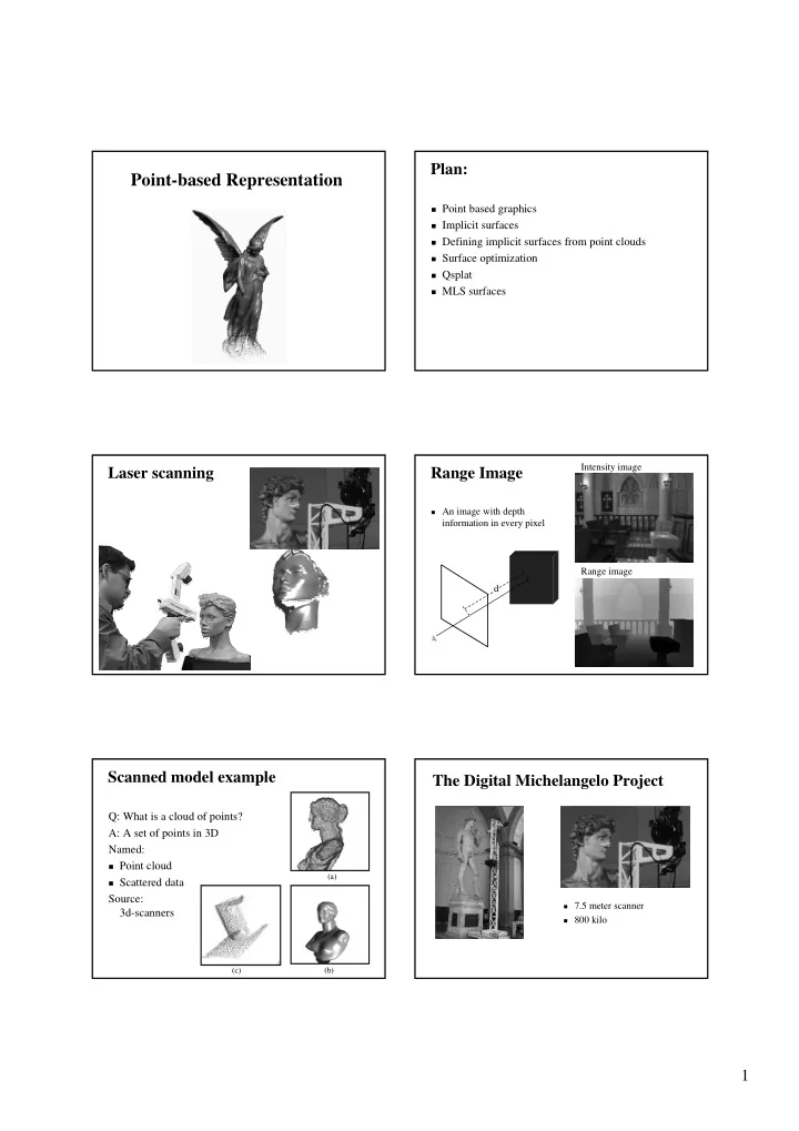
Point-based Representation Point based graphics Implicit surfaces - PDF document

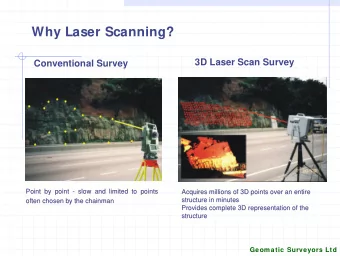
Plan: Point-based Representation � Point based graphics � Implicit surfaces � Defining implicit surfaces from point clouds � Surface optimization � Qsplat � MLS surfaces Intensity image Laser scanning Range Image � An image with depth information in every pixel Range image d Scanned model example The Digital Michelangelo Project Q: What is a cloud of points? A: A set of points in 3D Named: � Point cloud (a) � Scattered data Source: � 7.5 meter scanner 3d-scanners � 800 kilo (c) (b) 1

Statistics Large Polygonal model example � 1,080 man hours � 22 people � 480 scans � 2G polygons � 7000 Color images 1M � 32 Gigabyte Motivation Surface definition Operate � Polygonal models are getting complex � � Render, hardware � If we see 1M polygons, every polygon contributes to a single � Store – compress / transmit pixel � Edit � Scanned models produce clouds of points ÷ multi-resolution ÷ Constructive Solid Geometry (CSG) � Noisy scans - Denosing ÷ Blend, merge � Ambiguities Properties � � Smooth, sharp features � Oversampled – Simplification � Manifold � Goal – surface representation � Local properties � Interpolating / approximating � Parametric: polygon mesh, higher degree � Differential properties: normal… � Implicit functions � Noise handling � New types, direct methods � Parameterization Approximating Interpolating Smooth Sharp Feature Noise 2

Ambiguities Surface representations � Parametric � Polygonal meshes � Splines � Implicit functions (a) � Other, ad-hoc, MLS (b) Polygonal mesh Polygonal mesh Traditional computer graphics � Editing uses polygonal mesh as object � Hard to edit – self intersection representation � CSG � Well studied � High resolution models – � Hardware rendering overkill � Surface is well defined � Only piecewise smooth � Geometry � Topology � Color and texture Implicit functions Implicit functions r =0 � F(x,y) = 0 � Pros � F(x,y) = x 2 +y 2 -r 2 � Smooth <0 � CSG � Discrete form: image that >0 � Blend samples the function � Fill holes � Signed distance function: � Differential properties F(x,y) = ||<x,y> ; F -1 (0)|| � Cons For example 2 2 F ( x , y ) x y r � � � � Direct rendering, real-time rendering � Sharp features � Hard to parameterize 3

Normals Plane – sample X’ N � Surface normal usually gradient of function � Plane bounds half-space f > 0 � Specify plane with point p �� f ( x , y , z ) = ( � f / � x , � f / � y , � f / � z ) p and normal N x � Gradient not necessarily unit length � Points in plane x are perp. f < 0 � Gradient points in direction of increasing f to normal N f ( x ) = ( x - p ) � N � f is distance if || N || = 1 The point-surface CSG (constructive Solid Geometry) modeling pipeline Union(F,G)(x,y) = min(F(x,y), G(x,y)) Range Image Intensity Image � Intersection(F,G)(x,y) = max(F(x,y), G(x,y)) � Texture to Complement(F) = -F Registration � Geometry Subtract(F,G) = intersect(F,-G) � Error union intersect difference Compensation Meshing Simplification Texture maps Model Registration Marching cubes (Lorensen and Cline) Extracts a polygonal iso-surface from a signed distance function � Use pattern rules (configurations) in in in in in out out out 4

What is Marching Cubes? Forms a consistence surface � Volume is subdivided into unit cubes, which are analyzed and replaced by an appropriate set of - - - + + polygons � Threshold value marks points inside / outside - - - + + - - - + + - + + - + + - - - - - - - - - - - + - - + + - + + - - - + - + + + + - + - + - + - + - + + - + + - - + - + - + - + - - - - + + - + + + + + + + + + + MC ambiguities out in out in out in out in In 3D there are more configurations and more ambiguities. Configurations Simple results • 2^8=256 possible configurations (for a voxel), reduced to 15 (symmetry and rotations) Each configuration results in 1-4 � triangles being added to the isosurface The isosurface vertices can be � computed by: � Interpolation along edges (according to pixel values) – better shading, smoother surfaces � Default - middle of the edge. 5

Brain data set Voxilla Resolution Surface reconstruction from unorganized points [Hoppe94] Surface reconstruction from Surface Reconstruction unorganized points [Hoppe94] Surface U Points {x i } Initial Surface Estimation Mesh Optimization Given: points P sampled from Goal: reconstruct a surface unknown surface U S approximating U Smooth subdivision 6

Initial surface estimation Tangent plane estimation � Input: set of points {x i } � Compute n i that minimizes D U � Goal: Contour tracing p x n � � � � (Marching cubes) � j i i Nbhd(x i ) p - j Where � Estimate signed distance n i function d U :D � IR p � Nbhd x � � j i � Associate an oriented plane x i + with each point {x i } � Create a globally consistent orientation Consistent tangent plane orientation Signed distance function � Assumption: � d u (p) is the distance to the n tangent plane of the closest � if x i and x k are close then n x k n i and n k are nearly parallel point. x i k � If (n k · n i < 0) Flip n k i n k x k n i n k x i n k n i x k d u (p) x i p 3-Phase Reconstruction Results of Three Phases Goals: Determine the topological type of the surface Improve mesh’s accuracy and conciseness Points Phase 1 Phase 2 Find piecewise smooth surface fitting on the data Phase 3 7

Phase 1: Initial Surface Estimation Results of phase 1 From points to mesh: � Inferring topological type � Creating geometric approximation � Points (4,102) Initial Mesh (886 vertices) Phase 2: Phase 2: Mesh optimization Mesh Optimization � Optimize the energy function: � Optimization rules use edge collapse and expand E K , V E K , V E K E K , V � � � � � � � � � � � dist rep spring � Sum of square distances E K , V d ( x , K ) � � � � (accurate) � dist i i Phase 1 (886 vertices) Phase2 (163 vertices) � Number of vertices E K c K � (sparse) � � � � rep r � Regulation term � Input : data points P , initial mesh M initial � make vertices with E K , V c v v � Output: optimized mesh M, minimizing � � � � � � equidistance spring s j k j , k K � �  E ( M ) E E � � distance complexity Optimization steps Overview of Mesh Optimization Repeat (K ’ ,V ’ )=GenerateLegalMove(K,V) V ’ = OptVertexPosition(K ’ ,V ’ ) if E(K ’ ,V ’ ) < E(K,V) (K,V) = (K ’ , V ’ ) endif Until converges 8

Mesh Optimization results Mesh Optimization results Phase 3: Piecewise Smooth Surface Piecewise smooth � Not everywhere smooth, but piecewise smooth! Smooth surface Piecewise smooth surface Phase 3: Piecewise smooth subdivision Goal of Phase 3 surfaces � Perform optimization for Input the following: � Find a concise control mesh M: E K , L , V E E E � � � � � dist rep sharp � Same topological type as phase 2 � Optimization steps uses subdivision rules. � defining a piecewise smooth subdivision surface S(M) that accurately fits the points. Phase-3 K - mesh V - vertices L - sharp edges Phase-2 9

Subdivision Loop’s subdivision scheme Refinement procedure of splitting each triangular 2 � Subdivision is defined as: C face into four subfaces. “repeatedly refining a control mesh” � M=(K,V) � M 1 =R(M) � M 2 =R(R(M)) = R(M 1 ) Phase-3 Subdivision details Piecewise smooth subdivision surface � Not smooth everywhere! Subdivision mask � Creation of sharp features on surface: creases, n v v v � � 1 � � � r � � 0 1 n v � � corners and darts . 0 n n � � � � 3 3 v v v v � � � w r 1 � 0 2 2 4 � 1 Crease n n Corner � � � � v 1 Where 5 n � v 0 v 2 v 5 n 1 a n � � � � � n Smooth � � � � a n w 1 ’ w 3 ’ � � 2 5 3 2 cos 2 / 5 � � � � � � a n � � � � ’ v 4 Dart 8 64 v 3 w 2 The Result Phase-3 Results 1 2 M M S � M � The subdivision procedure 10

Point-based rendering Point-based rendering � What is the surface � Rendering the surface � What other operations are supported Projecting a point Projecting a point - reconstruction � A point is infinitely small � Splatting � Micro polygons � Image-space hole filling Rendering points – Hidden surface removal � Back to front Qsplat: A Multiresolution � Sort points: from nearest to farthest points Point Rendering System � Z-Buffer for Large Meshes � Arbitrary order Szymon Rusinkiewicz and Marc Levoy Stanford University 11