Abstract As a rule, developers of climate and biosphere models aim - PowerPoint PPT Presentation

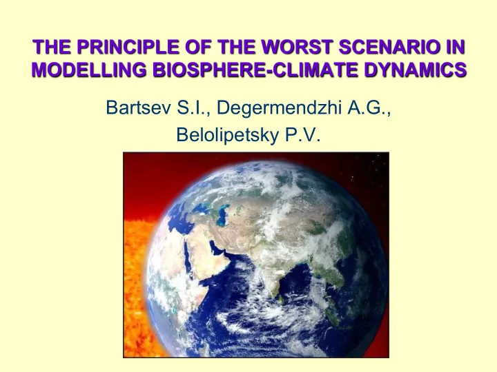
THE PRINCIPLE OF THE WORST SCENARIO IN MODELLING BIOSPHERE-CLIMATE DYNAMICS Bartsev S.I., Degermendzhi A.G., Belolipetsky P.V.

Abstract • As a rule, developers of climate and biosphere models aim at predicting the most probable scenario. Thus, they have to take into account the maximum possible number of various, frequently mutually compensating, interactions of the components of these systems. • However, assessment of the contribution of any climatic or biospheric process has finite accuracy and is represented by a confidence interval. So there are possible much large climatic and biosphere changes than in most probable scenario. • For the estimating probability of catastrophic changes we can seek not most probable scenario but just take parameters from the confidence intervals. (It is the idea of the principle of the worst scenario).

Forster, P., et al., 2007: Changes in atmospheric constituents and in radiative forcing, in Climate Change 2007: The Physical Science Basis. Contribution of Working Group I to the Fourth Assessment Report of the Intergovernmental Panel on Climate Change . Cambridge Univ. Press, Cambridge, U. K.

M.O. Andreae, C.D. Jones, P.M. Cox. 2005. Strong present day aerosol cooling implies a hot future. Nature. , 435 , 1187-1190.

Frequency distributions of T g (colours indicate density of trajectories per 0.1 K interval) through the three phases of the simulation D. A. Stainforth, T. Aina, C. Christensen, M. Collins, N. Faull, D. J. Frame, J. A. Kettleborough, S. Knight, A. Martin, J. M. Murphy, C. Piani, D. Sexton, L. A. Smith, R. A. Spicer, A. J. Thorpe & M. R. Allen Nature.-2005.-V.433.

Probability (%) of corresponding climate sensitivity. D. A. Stainforth, T. Aina, C. Christensen, M. Collins, N. Faull, D. J. Frame, J. A. Kettleborough, S. Knight, A. Martin, J. M. Murphy, C. Piani, D. Sexton, L. A. Smith, R. A. Spicer, A. J. Thorpe & M. R. Allen Nature.-2005.-V.433.

d T R Δ Δ C R f T f ∑ T = Δ + Δ Δ = − ∑ f i dt f i i i Roe and Baker. 2007. Why is climate sensitivity so unpredictable? Science, 318, 629–632.

R Δ f T 2 R 4 W m − Δ = − ∑ Δ = ⋅ f f i i longwave insolation feedback ⋅ o 2 1 f 3.2 W m C − − = − ⋅ I water vapour feedback 2 ⋅ o 1 f 1.8 0.18 W m C − − = ± ⋅ VW surface albedo feedback ⋅ o 2 1 f 0.26 0.08 W m C − − = ± ⋅ A cloud feedback ⋅ o 2 1 f 0.69 0.38 W m C − − = ± ⋅ C 2 ⋅ o 1 f 0.84 0.26 W m C − − Lapse rate feedback = ± ⋅ TG o T 3.1 C Δ = AVERAGE o o T 1.83 C T 10.26 C Δ = Δ = MIN MAX Randal, D. A., et al., 2007: Climate models and their evaluation, in Climate Change 2007: The Physical Science Basis. Contribution of Working Group I to the Fourth Assessment Report of the Intergovernmental Panel on Climate Change . Cambridge Univ. Press, Cambridge, U. K.

Denman, K.L., et al., 2007: Couplings between changes in the climate system and biogeochemistry, in Climate Change 2007: The Physical Science Basis. Contribution of Working Group I to the Fourth Assessment Report of the Intergovernmental Panel on Climate Change . Cambridge Univ. Press, Cambridge, U. K.

INITIAL MINIMAL MODEL OF GLOBAL CARBON DYNAMICS dC ⎧ Anthropogenic fuel ( t ) = ⎪ dt emissions ⎪ dx ⎪ P ( x , A , T ( A )) D ( x ) = − ⎪ dt ⎨ ⎪ Atmosphere dy D ( x ) S ( y , T ( A )) = − ⎪ dt ⎪ C A x y ⎪ = + + ⎩ A ⎛ ⎞ ( ) T A T T log ⎜ ⎟ = + ⋅ Terrestrial plants ⎜ ⎟ o del 2 A ⎝ ⎠ 0 P ( x , A ) V x ( x x ) V ( A ) f ( T ( A )) = ⋅ ⋅ − ⋅ ⋅ x max P d D ( x ) V x ( ) ( ) f T T T T = d ⋅ = − P P Soils S ( y , T ) V y f ( T ) = ⋅ ⋅ s M S.I. Bartsev, A.G. Degermendzhi, D.V. Erokhin. 2008. Principle of the worst scenario in the modelling past and future of biosphere dynamics. Ecological modelling. 216/2 , 160-171.

RESULTS OF INTIAL MINIMAL MODEL Atmosphere concentration СО 2, ppmv Dates Dynamics of atmosphere CO 2 at different dates of completely stopping the emission. - Mauna-Loa data; - 2059; - 2064; - 2070; - 2080.

INTEGRATED MINIMAL MODEL OF GLOBAL CARBON DYNAMICS S.I. Bartsev, A.G. Degermendzhi, D.V. Erokhin. 2008. Principle of the worst scenario in the modelling past and future of biosphere dynamics. Ecological modelling. 216/2 , 160-171.

VERIFICATION OF INTEGRATED MINIMAL MODEL 380 Atmosphere concentration СО 2 , ppmv 360 А ) 360 340 340 320 320 1960 1970 1980 1990 2000 . 300 280 1700 1750 1800 1850 1900 1950 2000 . Time, years Comparison of carbon dioxide dynamics by field data and numerical experiments. A) – comparison with Mauna-Loa meseurments.

RESULTS OF INTEGRATED MINIMAL MODEL 1100 22 1200 26 1100 18 1000 1000 24 1000 Температура, ¡ о С 17.5 20 Масса, ¡ГтС 900 900 800 22 17 В ) Б ) 800 18 800 600 20 А ) 16.5 700 700 400 18 16 16 600 600 200 16 500 15.5 500 14 0 14 2100 2200 2300 2100 2200 2300 2100 2200 2300 Time, ¡years Variants of scenarios for the development of the biosphere under different values of climate sensitivity parameter Т del : ( А ) – 2 о С ; ( Б ) – 4.5 о С ; ( В ) - 6 о С . In case ( В ) the irreversibility date is 2073 г . Solid line – biomass, dotted – dead organic matter, dashed – temperature.

Temperature influence on photosynthesis and soil respiration f(T) T opt T o C

The GCM is based on the third Hadley Centre coupled ocean-atmosphere model, HadCM3, coupled to an ocean carbon cycle model ( ‘‘ HadOCC ’’ ) and a dynamic global vegetation model ( ‘‘ TRIFFID ’’ ). P.M. Cox, R.A. Betts, M. Collins, P.P. Harris, C. Huntingford, C.D. Jones. 2004. Amazonian forest dieback under climate-carbon cycle projections for the 21 st century. Theor. Appl. Climatol. , 78 , 137-156.

Sufficient condition for runaway feedback dC T P S dt = − - gross primary production (GPP) P P f ( ) A f ( ) T = ⋅ ⋅ 0 F P - total respiration S S C f ( ) T = ⋅ ⋅ 0 T P P f ( ) A f ( ) T ⋅ ⋅ - equlibrium value of terrestrial eq C 0 F P = T S f T ( ) ⋅ carbon 0 S eq dC f ( ) A f ( ) T f T ( ) 1 T 1 1 ∂ ∂ ∂ ∂ eq T C ( F ( P S )) = + − T dA f ( ) A A A f ( ) T T f T ( ) T ∂ ∂ ∂ ∂ F P S

Sufficient condition for runaway feedback eq f T ( ) dC 1 f ( ) A T 1 f ( ) T 1 ∂ ∂ ∂ ∂ eq T C ( F ( P S )) = + − T dA f ( ) A A A f ( ) T T f T ( ) T ∂ ∂ ∂ ∂ F P S The land will tend to amplify CO2 induced climate change if terrestrial carbon decreases with increasing CO2 eq dC 0 T dA < The land would self-sustaining lose carbon to atmosphere, causing runaway feedback if: eq dC T (1 OceanUptake ) dA < − + There OceanUptake is a fraction of any increase in atmospheric carbon that the ocean takes-up

Summary • Mathematical models showing possibility of catastrophic changes were developed. Proposed parameterizations are not contradicting to field data, observations and experiments, parameters are from confidence intervals. • We introduced a notion of irreversible date – then concentration of CO 2 is so, that the land would self-sustaining lose carbon to the atmosphere even in the absence of anthropogenic emissions. • Sufficient condition for runaway feedback was estimated. • Experiments on closed laboratory ecosystems are carried out for investigating mechanisms used in models. • Minimal climate model based on the principle of the worst scenario is under development. It will be coupled with minimal biosphere model • It will be very interesting to investigate described effects using more complex models.

Thank you for attention

Эмпирическая зависимость роста среднегодовой глобально приповерхностной температуры от концентрации СО 2 (Gifford, 1993): A ⎛ ⎞ ( ) T A T T log ⎜ ⎟ = + ⋅ ⎜ ⎟ o del 2 A ⎝ ⎠ 0 где A – текущее количество углерода в атмосфере ; Ао – количество углерода в атмосфере в момент измерения среднегодовой приповерхностной температуры То , которая равна 15.5 ° C в настоящее время ; Т del – чувствительность климата .

Система уравнений модели имеет следующий вид : суша • Изменение количества углерода в биомассе живых растений : dx P ( x , A , T ( A )) D ( x ) = − dt • Динамика органических остатков : dy D ( x ) S ( y , T ( A )) = − dt