Abstract Subquadratic divide-and-conquer algorithms for computing - PowerPoint PPT Presentation

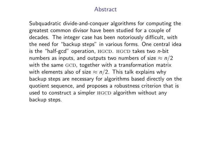
Abstract Subquadratic divide-and-conquer algorithms for computing the greatest common divisor have been studied for a couple of decades. The integer case has been notoriously difficult, with the need for “backup steps” in various forms. One central idea is the “half-gcd” operation, hgcd . hgcd takes two n -bit numbers as inputs, and outputs two numbers of size ≈ n / 2 with the same gcd , together with a transformation matrix with elements also of size ≈ n / 2. This talk explains why backup steps are necessary for algorithms based directly on the quotient sequence, and proposes a robustness criterion that is used to construct a simpler hgcd algorithm without any backup steps.

Subquadratic gcd Niels M¨ oller May 15, 2008

Outline Background Algorithm comparison The half-gcd (HGCD) operation Subquadratic hgcd Quotient based HGCD Jebelean’s criterion Why backup steps? Robust HGCD Simple subquadratic hgcd Difference-based hgcd Base case hgcd Further work

Background

History ◮ 300 BC (or even earlier): Euclid’s algorithm. ◮ 1938: Lehmer’s algorithm. ◮ 1961: Binary gcd described by Stein. ◮ 1994, 1995: Sorensson, Weber. ◮ 1970, 1971: Knuth and Sch¨ onhage, subquadratic computation of continued fractions. ◮ ca 1987: Sch¨ onhage’s “controlled Euclidean descent”, unpublished. ◮ 2004: St´ ehle and Zimmermann, recursive binary gcd . ◮ 2005–2008: M¨ oller. Left-to-right algorithm. Simpler and slightly faster than earlier algorithms.

Comparison of gcd algorithms Algorithm Time (ms) # lines 1440 304 gmp -4.1.4 (Weber) mpn gcd 87 1967 “Classical” Sch¨ onhage gcd mpn rgcd 93 1348 Rec. bin. (Stehl´ e/Zimmermann) mpn bgcd 100 760 1987 alg. (Sch¨ onhage/Weilert) mpn sgcd 85 733 New algorithm for gmp -5 mpn ngcd

Comparison of gcd algorithms Algorithm Time (ms) # lines 1440 304 gmp -4.1.4 (Weber) mpn gcd 87 1967 “Classical” Sch¨ onhage gcd mpn rgcd 93 1348 Rec. bin. (Stehl´ e/Zimmermann) mpn bgcd 100 760 1987 alg. (Sch¨ onhage/Weilert) mpn sgcd 85 733 New algorithm for gmp -5 mpn ngcd ◮ Benchmarked on 32-bit amd , with inputs of 48 000 digits. ◮ Cross-over around 7 700 digits.

Questions Q Where does the complexity come from? A Accurate computation of the quotient sequence. Q How to avoid that? A Stop bothering about quotients.

What is hgcd ? Definition (Reduction) � A � � α � = M B β ◮ Positive integers A , B , α , and β . ◮ Matrix M , non-negative integer elements. ◮ det M = 1.

What is hgcd ? Definition (Reduction) � A � � α � = M B β ◮ Positive integers A , B , α , and β . ◮ Matrix M , non-negative integer elements. ◮ det M = 1. Fact For any reduction, gcd ( A , B ) = gcd ( α, β )

What is hgcd ? Definition (Reduction) � A � � α � = M B β ◮ Positive integers A , B , α , and β . ◮ Matrix M , non-negative integer elements. ◮ det M = 1. Fact For any reduction, gcd ( A , B ) = gcd ( α, β ) Definition ( hgcd , “half gcd”) Input: A , B , of size n Output: M , with size of α , β and M elements ≈ n / 2

Main idea of subquadratic hgcd n p 1 . . A . . . B . � �� � M 1 ← hgcd ( ⌊ 2 − p 1 A ⌋ , ⌊ 2 − p 1 B ⌋ ) � A � � A � ← M − 1 1 B B ≈ 3 n / 4 p 2 . . . A . . B . � �� � M 2 ← hgcd ( ⌊ 2 − p 2 A ⌋ , ⌊ 2 − p 2 B ⌋ ) M ← M 1 · M 2

Asymptotic running time gcd ( A , B ) 1 while #( A , B ) > gcd-threshold 2 do 3 n ← #( A , B ), p ← ⌊ n / 2 ⌋ M ← hgcd ( ⌊ 2 − p A ⌋ , ⌊ 2 − p B ⌋ ) 4 ( A ; B ) ← M − 1 ( A ; B ) 5 6 return gcd-base ( A , B ) Running times for operations on n -bit numbers Multiplication: M ( n ) = O ( n log n log log n ) hgcd : H ( n ) = O ( M ( n ) log n ) gcd : G ( n ) ≈ 2 H ( n )

Quotient based HGCD

Definition (Quotient sequence) For any positive integers a , b , the quotient sequence q j and remainder sequence r j are defined by r 0 = a r 1 = b q j = ⌊ r j − 1 / r j ⌋ r j +1 = r j − 1 − q j r j

Definition (Quotient sequence) For any positive integers a , b , the quotient sequence q j and remainder sequence r j are defined by r 0 = a r 1 = b q j = ⌊ r j − 1 / r j ⌋ r j +1 = r j − 1 − q j r j Fact � a � � r j � = M b r j +1 with � q 1 � � q 2 � � q j � 1 1 1 M = · · · 1 0 1 0 1 0

Theorem (Jebelean’s criterion) Let a > b > 0 , with remainders r j and r j +1 , and � a � � u � � r j � u ′ = v ′ b v r j +1 � �� � = M Let p > 0 be arbitrary, 0 ≤ A ′ , B ′ < 2 p , and define � A � � a � � A ′ � = 2 p + B ′ B b � R j � � r j � � A ′ � = 2 p + M − 1 B ′ R j +1 r j +1 For even j, the following two statements are equivalent: (i) r j +1 ≥ v and r j − r j +1 ≥ u + u ′ (ii) For any p and any A ′ , B ′ , the jth remainders of A and B are R j and R j +1 . The quotient sequences are the same.

Theorem (Jebelean’s simplified criterion) Let a > b > 0 , with remainders r j , r j +1 and r j +2 , and � a � � r j � = M b r j +1 Assume that # r j +2 > ⌈ n / 2 ⌉ , with n = # a. Let p > 0 be arbitrary, 0 ≤ A ′ , B ′ < 2 p , and define � A � � a � � A ′ � = 2 p + B ′ B b � R j � � r j � � A ′ � + M − 1 = 2 p B ′ R j +1 r j +1 Then the jth remainders of A and B are R j and R j +1 . The quotient sequences are the same.

Quotient based hgcd A generalization of Lehmer’s algorithm Define hgcd ( a , b ) to return an M satisfying Jebelean’s criterion. Example (Recursive computation) ( a ; b ) = (858 824; 528 747) M 1 = (13 , 8; 8 , 5) No difficulties ( c ; d ) = M − 1 1 ( a ; b ) = 16 (4009; 194) + (0; 15) M 2 = hgcd (4009 , 194) = (21 , 20; 1 , 1) M − 1 2 (4009; 194) = (129; 65) Satisfies Jebelean M = M 1 · M 2 = (281 , 268; 173 , 165) M − 1 ( a ; b ) = (1764; 1355)

Backup step Example (Continued) ( a ; b ) = (858 824; 528 747) M = M 1 · M 2 = (281 , 268; 173 , 165) M − 1 ( a ; b ) = (1764; 1355) Violates Jebelean M corresponds to quotients 1 , 1 , 1 , 1 , 1 , 1 , 20 , 1. E.g., ( A ; B ) = 8 ( a ; b ) + (1; 7) has quotient sequence starting with 1 , 1 , 1 , 1 , 1 , 1 , 20 , 2.

Backup step Example (Continued) ( a ; b ) = (858 824; 528 747) M = M 1 · M 2 = (281 , 268; 173 , 165) M − 1 ( a ; b ) = (1764; 1355) Violates Jebelean M corresponds to quotients 1 , 1 , 1 , 1 , 1 , 1 , 20 , 1. E.g., ( A ; B ) = 8 ( a ; b ) + (1; 7) has quotient sequence starting with 1 , 1 , 1 , 1 , 1 , 1 , 20 , 2. Conclusion ◮ The quotients are correct for ( a ; b ), but not robust enough. ◮ Must drop final quotient before returning hgcd ( a , b ).

Robust HGCD

A robustness condition Definition (Robust reduction) A reduction M of ( A ; B ) is robust iff �� A � � x �� M − 1 + > 0 B y for all “small” ( x ; y ). More precisely, for all ( x ; y ) ∈ S , where S = { ( x ; y ) ∈ R 2 , | x | < 2 , | y | < 2 , | x − y | < 2 }

A robustness condition Definition (Robust reduction) A reduction M of ( A ; B ) is robust iff �� A � � x �� M − 1 + > 0 B y for all “small” ( x ; y ). More precisely, for all ( x ; y ) ∈ S , where S = { ( x ; y ) ∈ R 2 , | x | < 2 , | y | < 2 , | x − y | < 2 } Theorem The reduction � A � � u � � α � u ′ = v ′ β B v � �� � = M is robust iff α ≥ 2 max( u ′ , v ′ ) and β ≥ 2 max( u , v )

hgcd based on robustness hgcd ( A , B ) 1 n ← #( A , B ) 2 p 1 ← ⌊ n / 2 ⌋ M 1 ← hgcd ( ⌊ 2 − p 1 A ⌋ , ⌊ 2 − p 1 B ⌋ ) 3 ( C ; D ) ← M − 1 4 1 ( A ; B ) ✄ # | C − D | ≈ 3 n / 4 5 One subtraction and one division step on ( C ; D ). Update M 1 . 6 p 2 ← # M 1 + 2 M 2 ← hgcd ( ⌊ 2 − p 2 C ⌋ , ⌊ 2 − p 2 D ⌋ ) 7 8 return M 1 · M 2

hgcd based on robustness hgcd ( A , B ) 1 n ← #( A , B ) 2 p 1 ← ⌊ n / 2 ⌋ M 1 ← hgcd ( ⌊ 2 − p 1 A ⌋ , ⌊ 2 − p 1 B ⌋ ) 3 ( C ; D ) ← M − 1 4 1 ( A ; B ) ✄ # | C − D | ≈ 3 n / 4 5 One subtraction and one division step on ( C ; D ). Update M 1 . 6 p 2 ← # M 1 + 2 M 2 ← hgcd ( ⌊ 2 − p 2 C ⌋ , ⌊ 2 − p 2 D ⌋ ) 7 8 return M 1 · M 2 c = ⌊ 2 − p 2 C ⌋ c = 2 − p 2 C − c � �� A � � x �� � � c � �� � � x � � c M − 1 = 2 p 2 M − 1 + 2 − p 2 M − 1 + + � 2 1 B y d d y � �� � disturbance ∈ S

Strong robustness Definition (Strong robustess) Let n = #( A , B ) denote the bitsize of the larger of A and B . If # min( α, β ) > ⌊ n / 2 ⌋ + 1, then M is strongly robust. Lemma If a reduction M is strongly robust, then it is robust.

Strong robustness Definition (Strong robustess) Let n = #( A , B ) denote the bitsize of the larger of A and B . If # min( α, β ) > ⌊ n / 2 ⌋ + 1, then M is strongly robust. Lemma If a reduction M is strongly robust, then it is robust. Theorem (Sch¨ onhage-Weilert reduction) For arbitrary A , B > 0 , let n = #( A , B ) and s = ⌊ n / 2 ⌋ + 1 . Assume # min ( A , B ) > s. There exists a unique strongly robust M such that # min( α, β ) > s and # | α − β | ≤ s.