Ability Bias, Errors in Variables and Sibling Methods James J. - PowerPoint PPT Presentation
Ability Bias, Errors in Variables and Sibling Methods James J. Heckman University of Chicago Econ 312 This draft, May 26, 2006 1 1 Ability Bias Consider the model: log = 0 + 1 + where =
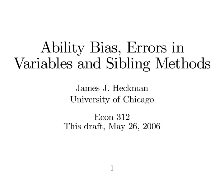
Ability Bias, Errors in Variables and Sibling Methods James J. Heckman University of Chicago Econ 312 This draft, May 26, 2006 1
1 Ability Bias Consider the model: log � �� = � 0 + � 1 � � + � �� where � �� = income, � � = schooling, and � 0 and � 1 are pa- rameters of interest. What we have omitted from the above specification is unobserved ability, which is captured in the residual term � �� . We thus re-write the above as: log � �� = � 0 + � 1 � � + � � + � �� where � � is ability, ( � �� � � � 0 � ) � � ( � � � � � 0 ) , and we believe that ��� ( � � � � � ) 6 = 0 . Thus, � ( � �� | � � ) 6 = 0 , so that OLS on our original specification gives biased and inconsistent estimates. 2
1.1 Strategies for Estimation 1. Use proxies for ability : Find proxies for ability and in- clude them as regressors. Examples may include: height, weight, etc. The problem with this approach is that prox- ies may measure ability with error and thus introduce additional bias (see Section 1.3). 3
2. Fixed E � ect Method : Find a paired comparison. Exam- ples may include a genetic twin or sibling with similar or identical ability. Consider two individuals � and � 0 : ( � 0 + � 1 � � + � �� ) � ( � 0 + � 1 � � 0 + � � 0 � ) log � �� � log � � 0 � = = � 1 ( � � � � � 0 ) + ( � � � � � 0 ) + ( � �� � � � 0 � ) Note: if � � = � � 0 , then OLS performed on our fixed e � ect 4
estimator is unbiased and consistent. If � � 6 = � � 0 , then we just get a di � erent bias (see Section 1.2). Further, if � � is measured with error, we may exacerbate the bias in our fixed e � ect estimator (see Section 1.3). 1.2 OLS vs. Fixed E � ect (FE) In the OLS case with ability bias, we have: ) = � 1 + ��� ( �� � ) plim ( � ��� 1 � �� ( � ) (See derivation of Equation (2.2) for more background on the above derivation). 5
We also impose: 0 ) � �� ( � ) = � �� ( � ��� ( � 0 � � 0 ) ��� ( �� � ) = ��� ( � 0 � � ) ��� ( �� � 0 ) = With these assumptions, our fixed e � ect estimator is given by: � 1 + ��� ( � � � 0 � ( � � � 0 ) + ( � � � 0 )) plim � �� = 1 � �� ( � � � 0 ) � 1 + ��� ( �� � ) � ��� ( � 0 � � ) = � �� ( � ) � ��� ( �� � 0 ) . Note that if ��� ( � 0 � � ) = 0 � and ability is positively correlated with schooling, then the fixed e � ect estimator is upward biased. 6
From the preceding, we see that the fixed e � ect estimator has more asymptotic bias if: ��� ( �� � ) � ��� ( � 0 � � ) 0 ) � ��� ( �� � ) � �� ( � ) � ��� ( �� � � �� ( � ) � ��� ( � 0 � � ) � ��� ( �� � ) 0 ) . � �� ( � ) ��� ( �� � 7
1.3 Measurement Error Say � � = � + �� where � � is observed schooling. Our model now becomes: log � = � 0 + � 1 � + � = � 0 + � 1 � � + ( � + � � � 1 � ) and the fixed e � ect estimator gives: ( � 0 + � 1 � + � ) � ( � 0 + � 1 � 0 + � 0 ) log � � log � 0 = 0 ) + ( � � � 0 ) + � 1 ( � 0 � � ) = � 1 ( � � � � � Now we wish to examine which estimator ( OLS or fixed e � ect), has more asymptotic bias given our measurement error prob- lem. For the remaining arguments of this section, we assume: � ( � | � ) = � ( � 0 | � ) = � ( � | � 0 ) = 0 so that the OLS estimator gives: 8
��� � 1 + ��� ( � � � � + � � � 1 � ) plim � ��� = 1 � �� ( � � ) � 1 + ��� ( �� � ) � � 1 � �� ( � ) = . � �� ( � ) + � �� ( � ) The fixed e � ect estimator gives: ³ ´ 0 � ( � � � 0 ) + � 1 ( � 0 � � ) � � � � � plim � �� = � 1 + 1 � �� ( � � � � � 0 ) � 1 + ��� (( � � � 0 ) � ( � � � 0 )) � � 1 � �� ( � 0 � � ) = � �� ( � � � 0 ) + � �� ( � 0 � � ) � 1 + ��� ( �� � ) � ��� ( �� � 0 ) � � 1 � �� ( � ) = . 0 � � ) � �� ( � ) + � �� ( � ) � ��� ( � 9
Under what conditions will the fixed e � ect bias be greater? From the above, we know that this will be true if and only if: ��� ( �� � ) � ��� ( �� � 0 ) � � 1 � �� ( � ) � ��� ( �� � ) � � 1 � �� ( � ) � �� ( � ) + � �� ( � ) � ��� ( � 0 � � ) � �� ( � ) + � �� ( � ) � ��� ( �� � 0 ) ( � �� ( � ) + � �� ( � )) � ( � 1 � �� ( � ) � ��� ( �� � )) ��� ( � 0 � � ) � ��� ( �� � 0 ) � ��� ( �� � ) � � 1 � �� ( � ) 0 � � ) . � �� ( � ) + � �� ( � ) ��� ( � If this inequality holds, taking di � erences can actually worsen the fit over OLS alone. Intuitively, we see that we have di � er- enced out the true component, � , and compounded our mea- surement error problem with the fixed e � ect estimator. 10
� In the special case � = � 0 , the condition is � �� ( � ) + � �� ( � ) � ��� ( � 0 � � ) � ��� ( �� � ) � � 1 � �� ( � ) � � 1 � �� ( � ) � �� ( � ) + � �� ( � ) 11
� � � � 2 Errors in Variables 2.1 The Model Suppose that the equation for earnings is given by: � � = � 1 � � 1 + � 2 � � 2 + � � where � ( � � | � 1 � � � 2 � ) = 0 � �� � 0 . Also define: 1 � = � 1 � + � 1 � and 2 � = � 2 � + � 2 � � 12
Here, � � 1 � and � � 2 � are observed and measure � 1 � and � 2 � with error. We also impose that � � � � � � � �� � . So, our initial model can be equivalently re-written as: � � = � � 1 � � 1 + � � 2 � � 2 + ( � � � � 1 � � 1 � � 2 � � 2 ) . Finally, by assumed independence of � and � , we write: � � � = � � + � � . 13
2.2 McCallum’s Problem Question: Is it better for estimation of � 1 to include other vari- ables measured with error? Suppose that � 1 � is not measured with error, in the sense that � 1 � = 0 � while � 2 � is measured with error. In 2.2.1 and 2.2.2 below, we consider both excluding and including � 2 � � and investigate the asymptotic properties of both cases. 2.2.1 Excluded � 2 � The equation for earnings with omitted � 2 is: � = � 1 � 1 + ( � + � 2 � 2 ) 14
� � � Therefore, by arguments similar to those in the appendix, we know: plim ˜ � 1 = � 1 + � 12 � 2 . (2.1) � 11 Here, � 12 is the covariance between the regressors, and � 11 is the variance of � 1 � Before moving on to a more general model for the inclusion of � 2 � � let us first consider the classical case for including both variables. Suppose ¸ ¸ � � � � � 11 0 0 11 � � = � � � = . 0 0 � 22 22 We know that: £ ¤ � � ( � � � ) � 1 ( � � ) plim ˆ � = (2.2) 15
� � � � � � � � � � � � where the coe � cient and regressor vectors have been stacked appropriately (see Appendix for derivation). Note that � � rep- resents the variance-covariance matrix of the measurement er- rors, and � � is the variance-covariance matrix of the regressors. Straightforward computations thus give: plim ˆ " ¸# � � 1 ¸ � 1 � � � ¸ � � 11 + � � 0 0 11 11 = 0 � 22 + � � 0 22 22 � 2 � 11 ¸ 0 � � 1 � 11 + � � = 11 � 22 0 � 2 � 22 + � � 22 16
� � � � � � � � � � � � � � � 2.2.2 Included � 2 � In McCallum’s problem we suppose that � � 12 = 0 � Further, as � 1 � is not measured with error, � � 11 = 0 � Substituting this into equation 2.2 yields: ¸ � 1 � 0 ¸ � � 11 0 plim ˆ � 12 � = � � � 22 + � � 0 � 12 22 22 With a little algebra, the above gives: μ � 12 ¶ plim ˆ 22 = � 1 + � 2 � 1 22 � � 2 � 11 12 � 22 + � � � 11 μ � 12 ¶ μ ¶ 22 = � 1 + � 2 � 22 (1 � � 2 12 ) + � � � 11 22 17
� 2 12 where � 2 12 is simply the correlation coe � cient, � Further, � 11 � 22 we know that: 0 � � 2 12 � 1 so including � 2 � results in less asymptotic bias (inconsistency). (We get this result by comparing the above with the bias from excluding � 2 � in section 2.2.1, the result captured in equation (2.1)). So, we have justified the kitchen sink approach. This result generalizes to the multiple regressor case - 1 badly mea- sured variable with � good ones (Econometrica, 1972). 18
Recommend
More recommend
Explore More Topics
Stay informed with curated content and fresh updates.
