A smoothing majorization method for l 2 2 - l p p matrix minimization - PowerPoint PPT Presentation

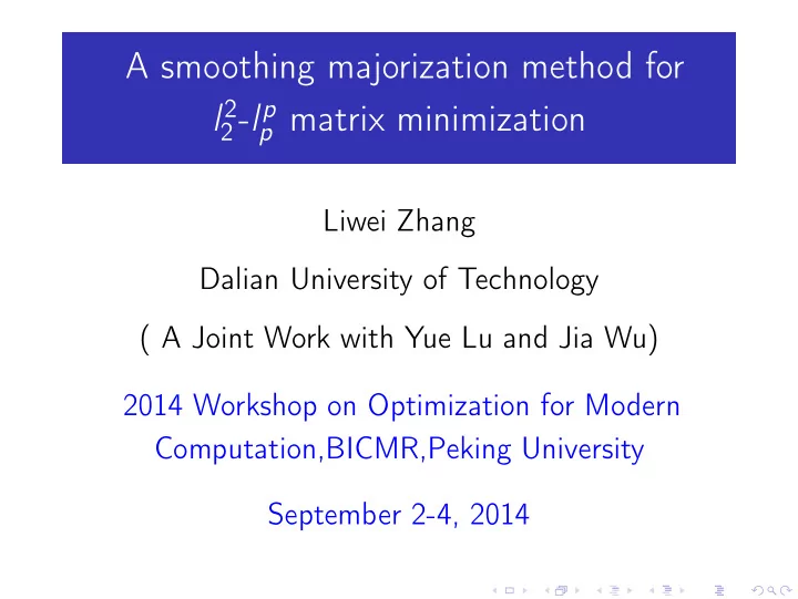
A smoothing majorization method for l 2 2 - l p p matrix minimization Liwei Zhang Dalian University of Technology ( A Joint Work with Yue Lu and Jia Wu) 2014 Workshop on Optimization for Modern Computation,BICMR,Peking University September 2-4, 2014

Introduction Lower bound analysis The smoothing model The majorization algorithm Numerical experiments Contents 1 Introduction 2 Lower bound analysis 3 The smoothing model 4 The majorization algorithm 5 Numerical experiments 2 / 55

Introduction Lower bound analysis The smoothing model The majorization algorithm Numerical experiments Background The aim of the matrix rank minimization problem is to find a matrix with minimum rank that satisfies a given convex constraint, i.e., min rank ( X ) (1) s.t. X ∈ C , where C is a nonempty closed convex subset of R m × n and R m × n represents the space of m × n matrices. 3 / 55

Introduction Lower bound analysis The smoothing model The majorization algorithm Numerical experiments Without loss of generality, we assume m ≤ n throughout this paper. For solving (1), Fazel et al. [13, 14] suggested using the matrix nuclear norm to approximate the rank function and proposed the following convex optimization problem min � X � ∗ (2) s.t. X ∈ C , where � X � ∗ := � m i = 1 σ i ( X ) , σ i ( X ) denotes the i th largest singular value of X . 4 / 55

Introduction Lower bound analysis The smoothing model The majorization algorithm Numerical experiments Many important problems can be formulated as (2). For example, several authors have used (2) to solve the famous matrix completion problem with the following model min � X � ∗ (3) s.t. X ij = M ij , ( i , j ) ∈ Ω , where Ω is an index set of the entries of M . the singular value thresholding algorithm [5], the fixed-point continuation algorithm [23], the alternating-direction-type algorithm [15]. 5 / 55

Introduction Lower bound analysis The smoothing model The majorization algorithm Numerical experiments Recently, these methods have also been applied to the nuclear norm regularized linear least square problem � 1 � 2 �A ( X ) − b � 2 min 2 + τ � X � ∗ , (4) X ∈ R m × n where A is a linear operator from R m × n to R q . It is worthwhile to note that (4) is regarded as a convex approximation to the regularized version of the affine rank minimization problem � 1 � 2 �A ( X ) − b � 2 min 2 + τ · rank ( X ) . (5) X ∈ R m × n 6 / 55

Introduction Lower bound analysis The smoothing model The majorization algorithm Numerical experiments The l 2 2 - l p p model We consider another approximation to (5), which uses the following l 2 2 - l p p model � � F ( X ) := 1 2 + τ 2 �A ( X ) − b � 2 p � X � p min , (6) p X ∈ R m × n p := � r i = 1 σ p where � X � p i ( X ) , r := rank ( X ) , p ∈ ( 0 , 1 ) and b ∈ R q . 7 / 55

Introduction Lower bound analysis The smoothing model The majorization algorithm Numerical experiments Vector model � 1 2 + τ � 2 � Cx − b � 2 p � x � p min . (7) p x ∈ R m X. J. Chen, F. Xu, and Y. Y. Ye, Lower bound theory of nonzero entries in solutions of l 2 -l p minimization , SIAM J. Sci. Comput., 32 (2011), pp. 2832–2852. X. J. Chen, Smoothing methods for nonsmooth, nonconvex minimization , Math. Program., 134 (2012), pp. 71–99. X. J. Chen, D. D. Ge, Z. Z. Wang and Y. Y. Ye, Complexity of unconstrained l 2 -l p minimization , Math. Program., 143 (2014), pp. 371–383. 8 / 55

Introduction Lower bound analysis The smoothing model The majorization algorithm Numerical experiments On vector l 2 2 - l p p problem Chen, Xu and Ye (2011) [10] gave a lower bound estimate of nonzero entries in solutions of (7). Chen (2012)[9] introduced the smoothing technique to tackle the term � x � p p and proposed an SQP-type algorithm to solve (7). Chen, Ge, Wang and Ye (2014) [11] studied the 2 - l p complexity of (7) and proved that the vector l 2 p problem (7) is strongly NP-Hard. 9 / 55

Introduction Lower bound analysis The smoothing model The majorization algorithm Numerical experiments The purpose of the work To check whether we can develop the parallel lower bound analysis in Chen, Xu and Ye (2011) [10] for the matrix l 2 2 - l p p problem. To develop an numerical method for solving an 2 - l p approximate solution to the matrix l 2 p problem. 10 / 55

Introduction Lower bound analysis The smoothing model The majorization algorithm Numerical experiments Features of the proposed method We present a smoothing majorization method in which the smoothing parameter ǫ is treated as a decision variable and introduce an automatic update mechanism of the smoothing parameter ǫ . The unconstrained subproblems based on the majorization functions are solved inexactly and the corresponding optimal solutions can be obtained explicitly. Numerical experiments show that our method is insensitive to the choice of the parameter p . 11 / 55

Introduction Lower bound analysis The smoothing model The majorization algorithm Numerical experiments Notations and definitions Given any X , Y ∈ R m × n , � X , Y � := Tr ( X T Y ) and the � Frobenius norm of X is denoted by � X � F := Tr ( XX T ) . Given any vector x ∈ R m , let x β := ( x β 1 , x β 2 , · · · , x β m ) T . For X ∈ R m × m , Diag ( X ) := ( X 11 , X 22 , · · · , X mm ) T . Given an index set I ⊆ { 1 , 2 , · · · , m } , x I denotes the sub-vector of x indexed by I . Similarly, X I denotes the sub-matrix of X whose columns are indexed by I . Denote the index I ( x ) := { j : j ∈ { 1 , 2 , · · · , m } and | x j | > 0 } for any x ∈ R m . 12 / 55

Introduction Lower bound analysis The smoothing model The majorization algorithm Numerical experiments Let X admit the singular value decomposition (SVD): � � V T , ( U , V ) ∈ O m , n ( X ) , X := U Diag ( σ ( X )) 0 m × ( n − m ) where σ 1 ( X ) ≥ σ 2 ( X ) ≥ · · · ≥ σ m ( X ) ≥ 0. O m , n ( X ) is given by � ( U , V ) ∈ O m × O n : X = � O m , n ( X ) := , � � V T U Diag ( σ ( X )) 0 m × ( n − m ) where O m represents the set of all m × m orthogonal matrices. 13 / 55

Introduction Lower bound analysis The smoothing model The majorization algorithm Numerical experiments The definitions of A and A ∗ : A ( X ) := ( � A 1 , X � , � A 2 , X � , · · · , � A q , X � ) T A ∗ ( y ) := � q i = 1 y i A i , where A i ∈ R m × n , y ∈ R q . Let G : R m × n → R and X , H ∈ R m × n , the second-order a teaux derivative D 2 G ( X ) at X is defined as follows: G ˆ D G ( X + tH ) − D G ( X ) D 2 G ( X ) H := lim . t t ↓ 0 14 / 55

Introduction Lower bound analysis The smoothing model The majorization algorithm Numerical experiments Smoothing function Let Φ : R m × n → R be a continuous function. We call Φ : R + × R m × n → R a smoothing function of Φ , if ¯ ¯ Φ( µ, · ) is continuously differentiable in R m × n for any fixed µ > 0, and for any X ∈ R m × n , we have ¯ lim Φ( µ, Z ) = Φ( X ) . µ ↓ 0 , Z → X 15 / 55

Introduction Lower bound analysis The smoothing model The majorization algorithm Numerical experiments Necessary optimality conditions Definition For X ∈ R m × n and p ∈ ( 0 , 1 ) , X is said to satisfy the first-order necessary condition of (6) if A ( X ) T ( A ( X ) − b ) + τ � X � p p = 0 . (8) Also, X is said to satisfy the second-order necessary condition of (6) if �A ( X ) � 2 2 + τ ( p − 1 ) � X � p p ≥ 0 . (9) 16 / 55

Introduction Lower bound analysis The smoothing model The majorization algorithm Numerical experiments Lemma Let X ⋆ be a local minimizer of (6). Then, for any pair ( U ⋆ , V ⋆ ) ∈ O m , n ( X ⋆ ) , the vector z ⋆ := σ ( X ⋆ ) ∈ R m is a local minimizer of the following problem ϕ ( z ) := F ( U ⋆ [ Diag ( z ) 0 m × ( n − m ) ]( V ⋆ ) T ) min (10) z ∈ R m . s.t. Theorem Let X ⋆ be any local minimizer of (6). Then X ⋆ satisfies the conditions (8) and (9). 17 / 55

Introduction Lower bound analysis The smoothing model The majorization algorithm Numerical experiments Lower bound result 1 Theorem Let X ⋆ be any local minimizer of (6) satisfying F ( X ⋆ ) ≤ F ( X 0 ) for any given point X 0 ∈ R m × n and µ A := √ q max 1 ≤ i ≤ q � A i � F . Then, for any i ∈ { 1 , 2 , · · · , m } , we have 1 � � 1 − p τ σ i ( X ⋆ ) < L ( τ, µ A , X 0 , p ) := ⇒ σ i ( X ⋆ ) = 0 . � µ A 2 F ( X 0 ) In addition, the rank of X ⋆ is bounded by � pF ( X 0 ) � min m , . τ L ( τ, µ A , X 0 , p ) p 18 / 55

Introduction Lower bound analysis The smoothing model The majorization algorithm Numerical experiments Hence, if X 0 = 0 and � A i � F = 1 ( i = 1 , 2 , · · · , q ) , we obtain the following corollary: Corollary Let X ⋆ be any local minimizer of (6). Then, for any i ∈ { 1 , 2 , · · · , m } , we have 1 � τ � 1 − p σ i ( X ⋆ ) < L 1 ( τ, p ) := σ i ( X ⋆ ) = 0 . ⇒ √ q � b � 2 In addition, the rank of X ⋆ is bounded by min � p � b � 2 � m , . 2 2 τ L 1 ( τ, p ) p 19 / 55