A Semigroup Approach for Weak Approximations with an Application to - PowerPoint PPT Presentation

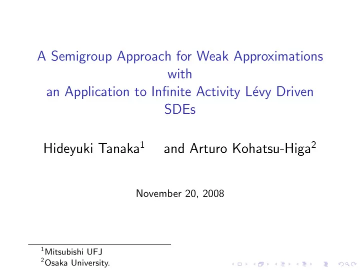
A Semigroup Approach for Weak Approximations with an Application to Infinite Activity L´ evy Driven SDEs Hideyuki Tanaka 1 and Arturo Kohatsu-Higa 2 November 20, 2008 1 Mitsubishi UFJ 2 Osaka University.

Abstract Weak approximations have been developed to calculate the expectation value of functionals of stochastic differential equations, and various numerical discretization schemes (Euler, Milshtein) have been studied by many authors. We present an operator decomposition method applicable to jump driven SDE’s. Setting & Goals Ideas from semigroup operators The algebraic structure First example: Coordinate processes General framework Weak approximation result Combination of ”coordinates” Examples: Diffusion, Levy driven SDE (Example: Tempered stable case)

Setting & Goals Setting � t � t � t ˜ X t ( x ) = x + V 0 ( X s − ( x )) ds + V ( X s − ( x )) dB s + h ( X s − ( x )) dY s . 0 0 0 (1) with C ∞ coefficients b V 0 : R N → R N , V = ( V 1 , . . . , V d ) , h : R N → R N ⊗ R d ˜ B t is a d -dim. BM and Y t is an d -dim. L´ evy with triplet ( b , 0 , ν ) satisfying the condition � (1 ∧ | y | p ) ν ( dy ) < ∞ . R d 0 for any p ∈ N . Goal Our purpose is to find discretization schemes ( X ( n ) ( x )) t =0 , T / n ,..., T t for given T > 0 such that T ( x ))] | ≤ C ( T , f , x ) | E [ f ( X T ( x ))] − E [ f ( X ( n ) . n m

Remarks ◮ 0a. Known general methods: Approximate by compounded Poisson (ignore small jumps). Protter, Talay, Kurtz, Meleard, Mordecki, Spessezy, et al. Adaptive Weak Approximation of Diffusions with Jumps E. Mordecki, A. Szepessy, R. Tempone and G. E. Zouraris

Remarks ◮ 0a. Known general methods: Approximate by compounded Poisson (ignore small jumps). Protter, Talay, Kurtz, Meleard, Mordecki, Spessezy, et al. Adaptive Weak Approximation of Diffusions with Jumps E. Mordecki, A. Szepessy, R. Tempone and G. E. Zouraris ◮ Questions (We are interested in stable like L´ evy measures.): 1a. Proof for Asmussen-Rosinski type approach 1b.Do we need to simulate all jumps if one wants an approximation of order 1 or 2? 1c.Limiting the number of jumps

Remarks ◮ 0a. Known general methods: Approximate by compounded Poisson (ignore small jumps). Protter, Talay, Kurtz, Meleard, Mordecki, Spessezy, et al. Adaptive Weak Approximation of Diffusions with Jumps E. Mordecki, A. Szepessy, R. Tempone and G. E. Zouraris ◮ Questions (We are interested in stable like L´ evy measures.): 1a. Proof for Asmussen-Rosinski type approach 1b.Do we need to simulate all jumps if one wants an approximation of order 1 or 2? 1c.Limiting the number of jumps ◮ 2. Proof through a ”semigroup type approach”

Remarks ◮ 0a. Known general methods: Approximate by compounded Poisson (ignore small jumps). Protter, Talay, Kurtz, Meleard, Mordecki, Spessezy, et al. Adaptive Weak Approximation of Diffusions with Jumps E. Mordecki, A. Szepessy, R. Tempone and G. E. Zouraris ◮ Questions (We are interested in stable like L´ evy measures.): 1a. Proof for Asmussen-Rosinski type approach 1b.Do we need to simulate all jumps if one wants an approximation of order 1 or 2? 1c.Limiting the number of jumps ◮ 2. Proof through a ”semigroup type approach” ◮ 3. Ideas come from Kusuoka type approximations S. Kusuoka. Approximation of expectation of diffusion processes based on Lie algebra and Malliavin calculus . Advances in mathematical economics. Vol. 6, 69-83, Adv. Math. Econ., 6, Springer, Tokyo, 2004.

Set-up for the proof of weak approximation Define: P t f ( x ) = E [ f ( X t ( x ))] Q t ≡ Q n t : operator such that the semigroup property is satisfied in { kT / n ; k = 0 , ..., n } . Q t ≈ P t in the sense that ( P t − Q t ) f ( x ) = O ( t m +1 ). Then the idea of the proof is n − 1 � P T f ( x ) − ( Q T / n ) n f ( x ) = ( Q T / n ) k ( P T / n − Q T / n ) P T − k +1 n T f ( x ) . k =0 For the proof to work we essentially need: Assumption R ( m , δ m ): The local difference P T / n − Q T / n has to be a ”small” operator. Assumption ( M ): The operators ( Q T / n ) k and P T − k +1 n T have to be stable. Next; We need to find a stochastic representation for Q and interpret the composition.

Simulation (stochastic characterization): Let M = M t ( x ) s.t. Q t f ( x ) = E [ f ( M t ( x ))]. Then Q T f ( x ) = ( Q T / n ) n f ( x ) = E [ f ( M 1 T / n ◦ · · · ◦ M n T / n ( x ))] Example: Euler-Maruyama scheme: M t ( x ) := x + ˜ V 0 ( x ) t + V ( x ) B t + h ( x ) Y t satisfies Assumption R ( m , δ m ): The local difference P T / n − Q T / n has to be a ”small” operator. Assumption ( M ): The operators ( Q T / n ) k and P T − k +1 n T have to be stable. Next: One has to be able to find stochastic representations for Q .

The algebraic structure m t k P t = e tL = k ! L k + O ( t m +1 ) � k =0 Note that L = � d +1 i =1 L i . m t k e tL i = � i + O ( t m +1 ) k ! L k k =0 Goal: Approximate e tL , through a combination of L i ’s s.t. k e tL − ξ j e t 1 , j A 1 , j · · · e t ℓ j , j A ℓ j , j = O ( t m +1 ) � j =1 with some t i , j > 0, A i , j ∈ { L 0 , L 1 , . . . , L d +1 } and weights { ξ j } ⊂ [0 , 1] with � k j =1 ξ j = 1. This will correspond to an m -th order discretization scheme.

First example: Coordinate processes Define the coordinate processes X i , t ( x ), i = 0 , ..., d + 1, solutions of � t X 0 , t ( x ) = x + V 0 ( X 0 , s ( x )) ds 0 � t V i ( X i , s ( x )) ◦ dB i X i , t ( x ) = x + s 1 ≤ i ≤ d 0 � t X d +1 , t ( x ) = x + h ( X d +1 , s − ( x )) dY s . 0 Define Q i , t f ( x ) := E [ f ( X i , t ( x ))] whose generators are L i f ( x ) := 1 2( V 2 L 0 f ( x ) := ( V 0 f )( x ) , i f )( x ) , 1 ≤ i ≤ d � L d +1 f ( x ) := ∇ f ( x ) h ( x ) b + ( f ( x + h ( x ) y ) − f ( x ) − ∇ f ( x ) h ( x ) τ ( y )) ν ( dy )

How does the algebraic argument work? For simplicity let d + 1 = 2 then e tL = I + tL + t 2 2 L 2 + O ( t 3 ) 2 L 2 ≈ ( I + tL 1 + t 2 1 + ... )( I + tL 2 + t 2 t t 2 L 1 e 2 L 2 2 L 2 e 2 + ... ) = I + tL + t 2 L 2 2 + L 2 + O ( t 3 ) � � 1 + L 1 L 2 2 then e tL − e t 2 L 2 = O ( t 2 ) t 2 L 1 e e tL − 1 2 L 2 − 1 t t t t 2 L 1 = O ( t 3 ) 2 L 1 e 2 L 2 e 2 e 2 e finally one needs to obtain a stochastic representation for t t t t 2 L 2 + 1 1 2 L 1 e 2 L 2 e 2 L 1 . 2 e 2 e

Examples of schemes: Ninomiya-Victoir (a) : 1 2 L 0 + 1 t t t t 2 L 0 e tL 1 · · · e tL d +1 e 2 L 0 e tL d +1 · · · e tL 1 e 2 L 0 2 e 2 e Ninomiya-Victoir (b) : 1 2 e tL 0 e tL 1 · · · e tL d +1 + 1 2 e tL d +1 · · · e tL 1 e tL 0 Splitting method : t t t t 2 L 0 · · · e 2 L d · · · e 2 L d e tL d +1 e 2 L 0 e So the idea is k � ξ j e t 1 , j A 1 , j · · · e t ℓ j , j A ℓ j , j f P t f = e tL f ≈ j =1 k � ≈ ξ j E [ f ( M 1 ( t 1 , j , M 2 ( t 2 , j , ( ...., M l ( t l , j , · )) ... ))] j =1

General framework Assumptions M ◮ If f ∈ C p with p ≥ 2, then Q t f ∈ C p and sup � Q t f � C p ≤ K � f � C p t ∈ [0 , T ] for K > 0 independent of n . Futhermore, we assume 0 ≤ Q t f ( x ) ≤ Q t g ( x ) whenever 0 ≤ f ≤ g .

General framework Assumptions M ◮ If f ∈ C p with p ≥ 2, then Q t f ∈ C p and sup � Q t f � C p ≤ K � f � C p t ∈ [0 , T ] for K > 0 independent of n . Futhermore, we assume 0 ≤ Q t f ( x ) ≤ Q t g ( x ) whenever 0 ≤ f ≤ g . ◮ For f p ( x ) := | x | 2 p ( p ∈ N ), Q t f p ( x ) ≤ (1 + Kt ) f p ( x ) + K ′ t for K = K ( T , p ), K ′ = K ′ ( T , p ) > 0.

General framework Assumptions M ◮ If f ∈ C p with p ≥ 2, then Q t f ∈ C p and sup � Q t f � C p ≤ K � f � C p t ∈ [0 , T ] for K > 0 independent of n . Futhermore, we assume 0 ≤ Q t f ( x ) ≤ Q t g ( x ) whenever 0 ≤ f ≤ g . ◮ For f p ( x ) := | x | 2 p ( p ∈ N ), Q t f p ( x ) ≤ (1 + Kt ) f p ( x ) + K ′ t for K = K ( T , p ), K ′ = K ′ ( T , p ) > 0. ◮ For m ∈ N , δ m : [0 , T ] → R + denotes a decreasing function s.t. δ m ( t ) lim sup t m − 1 = 0 . t → 0+ Usually, we have δ m ( t ) = t m .

Main hypothesis R ( m , δ m ) For p ≥ 2, there exists q = q ( m , p ) ≥ p and linear operators e k : C 2 k → C p +2 k ( k = 0 , 1 , . . . , m ) s.t. p with 1 ≤ m ′ ≤ m , the operator Q t (A): For every f ∈ C 2( m ′ +1) p satisfies m ′ ( e k f )( x ) t k + ( Err ( m ′ ) � Q t f ( x ) = f )( x ) , t ∈ [0 , T ] , (2) t k =0 where Err ( m ′ ) f ∈ C q , and satisfies the following condition: t with m ′′ ≥ 2 k , then e k f ∈ C m ′′ − 2 k (B): If f ∈ C m ′′ and there p p +2 k exists a constant constant K = K ( T , m ) > 0 such that � e k f � C m ′′− 2 k ≤ K � f � C m ′′ k = 0 , 1 , . . . , m . (3) p p +2 k with m ′′ ≥ 2 m ′ + 2, Furthermore if f ∈ C m ′′ p if m ′ < m Kt m ′ +1 � f � C m ′′ � � Err ( m ′ ) f � C q ≤ p if m ′ = m t Kt δ m ( t ) � f � C m ′′ p for all 0 ≤ t ≤ T .