A Quantitative Analysis of Subsidy Competition in the U.S. Ralph - PowerPoint PPT Presentation
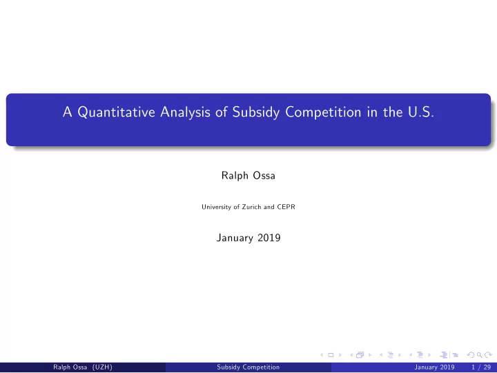
A Quantitative Analysis of Subsidy Competition in the U.S. Ralph Ossa University of Zurich and CEPR January 2019 Ralph Ossa (UZH) Subsidy Competition January 2019 1 / 29 Motivation and objectives Motivation US cities, counties, and states
A Quantitative Analysis of Subsidy Competition in the U.S. Ralph Ossa University of Zurich and CEPR January 2019 Ralph Ossa (UZH) Subsidy Competition January 2019 1 / 29
Motivation and objectives Motivation US cities, counties, and states spend substantial resources on subsidies trying to attract firms from other locations Such subsidies had an annual cost of $45 billion in 2015, equivalent to 30% of average state and local business taxes Objectives Understand what motivates regional governments to subsidize firm relocations and quantify how strong their incentives are Characterize fully non-cooperative and cooperative subsidy choices and assess how far away we are from these extremes Ralph Ossa (UZH) Subsidy Competition January 2019 2 / 29
Strategy and findings Strategy I pursue these objectives in the context of a quantitative economic geography model which I calibrate to US states I calculate optimal subsides, Nash subsidies, and cooperative subsidies and compare them to observed subsidies Findings I show that states have strong incentives to subsidize firm relocations in order to gain at the expense of other states Observed subsidies are closer to cooperative than non-cooperative subsidies but the potential losses from an escalation of subsidy competition are large Ralph Ossa (UZH) Subsidy Competition January 2019 3 / 29
Mechanism and approach Mechanism My model features agglomeration externalities in the New Economic Geography tradition which poli- cymakers try to exploit Consumers want to be close to firms and firms want to be close to firms to have better access to final and intermediate goods Approach I try to strike a balance between transparency and realism to be able to clearly illustrate the main mechanism and yet obtain broadly credible quantitative results Analytical results are notoriously hard to derive in economic geography models and the standard practice has been to resort to simple numerical examples instead Ralph Ossa (UZH) Subsidy Competition January 2019 4 / 29
Contribution I am not aware of any comparable analysis of noncooperative and cooperative policy in a spatial environment Theoretical work such as Baldwin et al (2005) restricts attention to highly stylized models and does not connect to data Quantitative work such as Gaubert (2014), Suarez Serrato and Zidar (2016), and Fajgelbaum et al (2016) takes policy as given My modeling of agglomeration forces builds on Krugman (1991), Krugman and Venables (1995), and Allen and Arkolakis (2014) Methodologically most similar are the recent contributions by Ossa (2014), Fajgelbaum et al (2016), and Redding (2016) Ralph Ossa (UZH) Subsidy Competition January 2019 5 / 29
Outline Model Calibration Analysis Ralph Ossa (UZH) Subsidy Competition January 2019 6 / 29
Model - Setup - Preferences Preferences are common over goods and heterogeneous over amenities: U jv = U j u jv � � µ � � 1 − µ T R C F A j j j U j = L j µ 1 − µ � � ε � M i ε − 1 ε − 1 C F ∑ c F = ij ( ω i ) ε d ω i j 0 i u jv ∼ Frechet ( 1 , σ ) NB: Heterogeneity is necessary to allow for a meaningful sense in which states can benefit at the expense of one another Ralph Ossa (UZH) Subsidy Competition January 2019 7 / 29
Model - Setup - Technology Firms produce differentiated products using labor, capital, land, and intermediates: q j = ϕ j ( z j − f j ) � θ T η � � θ K � � 1 − η � L j � θ L � K j T C C I 1 1 j j z j = M j η θ L θ K θ T 1 − η � � ε � M i ε − 1 ε − 1 C I ∑ c I = ij ( ω i ) ε d ω i j 0 i θ L + θ K + θ T 1 = NB: Tax-financed cost subsidies would not work if there was only labor because then workers would essentially subsidize themselves Ralph Ossa (UZH) Subsidy Competition January 2019 8 / 29
Model - Setup - Government Government objective In the non-cooperative regime, local governments maximize local expected utility, E ( U jv | living in j ) , which amounts to maximizing U j In the cooperative regime, the federal government maximizes national expected utility, E ( max j { U jv } ) , � � 1 σ ∑ R i = 1 U σ which amounts to maximizing i Policy instruments Governments provide cost subsidies to local firms which they finance with lump-sum taxes on local residents These subsidies capture deviations from a benefit tax benchmark which includes statutory corporate tax rates Ralph Ossa (UZH) Subsidy Competition January 2019 9 / 29
Model - Equilibrium - Properties The solution to the model can be expressed as a system of 4 N equilibrium conditions in the L K C 4 N unknows ˆ i , ˆ i , ˆ i , and ˆ λ λ λ P i It can be calibrated with minimal data requirements using the "exact hat algebra" approach of Dekle et al (2008) Following Allen and Arkolakis (2014), the model is isomorphic to an Armington model with 1 external IRS technology if φ = ε − 1 and the technology is: ϕ i ( Z i ) 1 + φ = Q i � θ T η � � θ K � � 1 − η � L i � θ L � K i T C C I 1 i i Z i = θ L θ K θ T 1 − η η Ralph Ossa (UZH) Subsidy Competition January 2019 10 / 29
Calibration - Data Business incentives databases of Bartik (2017) and Story et al (2012) s i = 0 . 5 % , s min = 0 . 0 % (CO), s max ¯ = 3 . 8 % (NM) Map i i 2007 Commodity Flow Survey T ij 2007 Annual Survey of Manufacturing λ L i 2007 BEA Input-Output Table and BLS Capital Income Table θ L = 0 . 57, θ K = 0 . 33, θ T = 0 . 10, η = 0 . 58 Earlier work including Suarez Serrato and Zidar (2015) and Redding (2015) σ = 1 . 2, µ = 0 . 25, ε = 5 Ralph Ossa (UZH) Subsidy Competition January 2019 11 / 29
Calibration - Adjustments I purge the trade data of the net exports due to nominal transfers so that subsidies cannot affect the real values of nominal transfers For this calculation, I work with a version of the model without labor mobility to preserve the original distribution of employment Details I also allow for a federal subsidy on differentiated goods purchases in order to isolate the beggar-thy-neighbor aspects of state subsidies Details � ( w i ) θ L ( i ) θ K ( r ) θ T � η � � 1 − η ρ i τ ij ρ F P i ε p ij = ε − 1 ϕ i Ralph Ossa (UZH) Subsidy Competition January 2019 12 / 29
Calibration - Multiplicity of equilibria Ralph Ossa (UZH) Subsidy Competition January 2019 13 / 29
Calibration - Model fit The calibration procedure essentially pins down trade costs, amenities, and productivities such that manufacturing trade and employment are exactly matched Assuming τ ij = τ ji and τ ii = 1, the model can be inverted and relative trade costs, amenities, and productivities can be backed out (as well as many other variables) It turns out that the variation in trade flows and manufacturing employment is mainly at- tributed to variation in trade costs and amenities, respectively Details Ralph Ossa (UZH) Subsidy Competition January 2019 14 / 29
Welfare effects of subsidy - Example F i g u r e 2: Effects of subsidy imposed by IL 0.5 0 0 IL local welfare change in % (left scale) Other local welfare change in % (right scale) -0.5 -5 0 5 10 15 Subsidy (in %) 50 2 0 0 IL variety change in % (left scale) Other variety change in % (right scale) -2 -50 -5 0 5 10 15 Subsidy (in %) 5.3 10 5.2 8 5.1 6 5 4 IL employment share in % (left scale) IL capital share in % (right scale) 4.9 2 4.8 0 -5 0 5 10 15 Subsidy (in %) Ralph Ossa (UZH) Subsidy Competition January 2019 15 / 29
Welfare effects of subsidy - Decomposition Under certain restrictions, the welfare effects resulting from small subsidy changes can be decomposed into: � � � dp j � � dr j � d λ L − d λ C dU j = 1 X ij 1 dM i + 1 X ij − dp i − dP j j j η ∑ η ∑ − θ T − µ λ L λ C U j E j ε − 1 M i E j p j p i r j P j i i j j � �� � � �� � � �� � � �� � residential congestion home market effect terms-of-trade effect commercial congestion The terms-of-trade effect can be further decomposed into: � � � dw j � � dr j � � dP j � d ρ j θ L ∑ X ij − dw i + θ T ∑ X ij − dr i + 1 X ij − d ρ i + 1 - η X ij − dP i η ∑ η ∑ E j w j w i E j r j r i E j ρ j ρ i E j P j P i i i i i � �� � � �� � � �� � � �� � relative wage effect relative rent effect intermediate cost effect direct subsidy effect For example, if IL unilaterally imposes a 5 percent subsidy, the approximate welfare effects are: U HME TOT CON TOT w TOT r TOT s TOT int CON res CON com - 2.1% IL 1.2% 1.6% 1.0% -1.4% 5.4% 0.5% -4.5% -0.3% 0.7% Ralph Ossa (UZH) Subsidy Competition January 2019 16 / 29
Optimal subsidies Figure 3: Optimal subsidies 13 LA WA CA OR 12 AZ TX FL CO MN UT IA NC 11 MA MI WI OK AL ME CT VA KS Optimal subsidy in % 10 NY MO GA OH AR PA IN SD ID MS 9 NE ND IL SC VT KY DE 8 NJ WY NV MD NH 7 NM WV RI 6 MT TN 5 15 20 25 30 35 40 45 50 55 60 65 Own trade share in % NB: Optimal subsidies average 9.6% or $14.9 billion Own trade share Ralph Ossa (UZH) Subsidy Competition January 2019 17 / 29
Recommend
More recommend
Explore More Topics
Stay informed with curated content and fresh updates.
