Chapter 5: Short Run Price Competition Price competition (Bertrand - PDF document

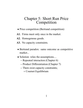
Chapter 5: Short Run Price Competition • Price competition (Bertrand competition) A1. Firms meet only once in the market. A2. Homogenous goods. A3. No capacity constraints. • Bertrand paradox: same outcome as competitive market... • Solution: relax the assumptions.... – Repeated interaction (Chapter 6) – Product Differentiation (Chapter 7) – There exist capacity constraints; ∗ Cournot Equilibrium 1

1 The Bertrand Paradox • Duopoly, n = 2 • Because identical goods, consumers buy from the supplier that charges the lowest price. • Market demand: q = D ( p ) • Marginal cost: c • Firm i ’s demand is   D ( p i ) if p i < p j   1 2 D ( p i ) if p i = p j D i ( p i , p j ) =    if p i > p j 0 • Firm i ’s pro fi t is Π i ( p i , p j ) = ( p i − c ) D i ( p i , p j ) De fi nition A Nash equilibrium in price ( Bertrand equilibrium ) is a pair of prices ( p ∗ 1 , p ∗ 2 ) such that each fi rm i ’s price maximizes the pro fi t of i , given the other fi rm’s price. Π i ( p ∗ i , p ∗ j ) ≥ Π i ( p i , p ∗ j ) for i = 1 , 2 and for any p i . 2

• The Bertrand Paradox (1883): The unique equilibrium is p ∗ 2 = c . 1 = p ∗ • Firms price at MC and make no pro fi t. • If asymmetric marginal costs c 1 < c 2 , it is no longer an equilibrium. – p = c 2 ( fi rm 1 sets price lower than c 2 to get the whole market) – fi rm 1 makes Π 1 = ( c 2 − c 1 ) D ( c 2 ) and fi rm 2 has no pro fi t. 3

2 Solutions to Bertrand Paradox 2.1 Repeated Interaction (relax A1) • Chapter 6 • If fi rms meet more than once, ( p ∗ 1 , p ∗ 2 ) = ( c, c ) is no longer an equilibrium. • Collusive behavior can be sustain by the threat of future losses in a price war. 2.2 Product Differentiation (relax A2) • Chapter 7 • With homogenous product: at equal price, consumers are just indifferent between goods. • If goods are differentiated: ( p ∗ 1 , p ∗ 2 ) = ( c, c ) is no longer an equilibrium. • Example: spacial differentiation 4

2.3 Capacity Constraints (relax A3) • Edgeworth solution (1887). • If fi rms cannot sell more than they are capable of producing: ( p ∗ 2 ) = ( c, c ) is no longer an equilibrium. 1 , p ∗ • Why? If fi rm 1 has a production capacity smaller than D ( c ) , fi rm 2 can increase his price and get a positive pro fi t. • Example: 2 hotels in a small town, number of beds are fi xed in SR. • The existence of a rigid capacity constraint is a special case of a decreasing returns-to-scale technology. • Why? Firm 1 has a marginal cost of c up to the capacity constraint and then MC = ∞ . 5

3 Decreasing Returns-to-scale and Capacity Constraints 3.1 Rationing rules • Cost of production C i ( q i ) is increasing and convex, C 0 i ( q i ) > 0 and C 00 i ( q i ) ≥ 0 , for any q i . • If fi rm 1 has a capacity constraint, there exists a residual demand for 2. It depends on the rationing rule. • p 1 < p 2 • Supply of fi rm 1 is q 1 = S 1 ( p 1 ) 3.1.1 The ef fi cient-rationing rule (parallel) • Suppose q 1 < D ( p 1 ) • Residual demand for fi rm 2 is ( D ( p 2 ) − q 1 if D ( p 2 ) > q 1 e D 2 ( p 2 ) = otherwise 0 • It is as if the most eager consumers buy from 1, others from 2. • Ef fi cient because maximizes consumers’ surplus. 6

3.1.2 The proportional-rationing rule (randomized) • All consumers have the same probability of being rationed. • Demand that cannot be satis fi ed at p 1 : D ( p 1 ) − q 1 • Thus fraction of consumers that cannot buy at p 1 (probability of not being able to buy from 1) is D ( p 1 ) − q 1 D ( p 1 ) • Residual demand for 2 is D 2 ( p 2 ) = D ( p 2 ) D ( p 1 ) − q 1 e D ( p 1 ) • Not ef fi cient for consumers. • However, fi rm 2 prefers this rule because his residual demand is higher for each price. 3.2 Price Competition • Decreasing returns-to-scale softens price competition. Both fi rms’ prices exceed the competitive price. • Demand function is D ( p ) = 1 − p • Inverse demand function is P = P ( q 1 + q 2 ) = 1 − q 1 − q 2 7

• The two fi rms have capacity constraints q i ≤ q i • Investment: c 0 ∈ [ 3 4 , 1] unit cost of acquiring the capacity q i . • Marginal cost of producing is 0 up to q i and then it is ∞ . • Rule is ef fi cient rationing rule. • Price that maximizes (gross) monopoly pro fi t Max p (1 − p ) p is p m = 1 / 2 and thus Π m = 1 / 4 . • Thus the (net) pro fi t of fi rm i is at most 1 / 4 − c 0 q i and is negative for q i ≥ 1 / 3 . • Assume that q i ∈ [0 , 1 / 3] • The unique Nash equilibrium is p ∗ = 1 − ( q 1 + q 2 ) • Proof: – Is it worth charging a lower price? NO because of the capacity constraints. – Is it worth charging a higher price? Pro fi t of i if price p ≥ p ∗ is Π i = q (1 − q − q j ) where q is the quantity 8

sold by fi rm i at price p . Furthermore ∂ Π i ∂ q = 1 − 2 q − q j and ∂ 2 Π i ∂ q 2 < 0 – For q = q i , 1 − 2 q i − q j > 0 as q i < 1 / 3 and q j < 1 / 3 . – Hence, increasing p above p ∗ is not optimal (i.e. lowering q below q i ). • It is as if the 2 fi rms produce at the capacities, and an auctioneer equals supply and demand. • For q i ∈ [0 , 1 / 3] , i = 1 , 2 , the fi rms’ reduced form pro fi t functions are the exact Cournot forms (Levitan and Shubik (1972)) • Gross Π ig ( q i , q j ) = (1 − ( q i + q j )) q i • Net Π ig ( q i , q j ) = (1 − ( q i + q j ) − c 0 ) q i • Same result with the proportional rationing rule (Beckman (1967)). 9

• The assumption of large investment cost insures small capacities, and thus we fi nd a solution. • For larger capacities : no equilibrium in pure strategies, only in mixed strategies . 3.3 Ex ante Investment and ex post price competition • A two stage-game in which 1. fi rms simultaneously choose q i 2. Firms observe the capacities and simultaneously choose p i . • is equivalent to a one-stage game in which fi rms choose quantities q i and an auctioneer determines the market price that clears the market p = P ( q 1 + q 2 ) ; Cournot (1838). • Examples of ex ante choice of scale: – Hotel (cannot adjust its capacity), – Vendor of perishable food. 10

4 Cournot Competition • Firms choose the quantities simultaneously. • Each fi rm maximizes his pro fi t Π i ( q i , q j ) = q i P ( q i + q j ) − C i ( q i ) • where Π i ( . ) is strictly concave in q i and twice differen- tiable. • FOC i : ∂ P ( . ) + P ( q i + q j ) − ∂ C i ( q i ) q i = 0 ∂ q i ∂ q i ⇒ q i = R i ( q j ) Best response function of i to q j • Lerner index is q i = α i Q $ i = − P 1 ε ∂ P ( . ) Q ∂ qi • where α i is fi rm i ’s market share . • Thus the Lerner index is – proportional to the fi rm’s market share, – inversely proportional to the elasticity of demand. 11

4.1 Case of linear demand Duopoly • P ( Q ) = 1 − Q • C i ( q i ) = c i q i • What are the reaction functions? R i ( q j ) = 1 − c i − q j 2 for i, j = 1 , 2 and i 6 = j. • What is the Cournot equilibrium? i = 1 − 2 c i + c j q ∗ 3 • What are the pro fi ts of the fi rms? Π i = (1 − 2 c i + c j ) 2 9 • A fi rm’s output decreases with its MC , ∂ q i ∂ c i < 0 . • A fi rm’s output increases with its competitor MC , ∂ q i ∂ cj > 0 . 12

• For more general demand and cost functions, these 2 conditions are true: a. If reaction curves are downward sloping (quantities are strategic substitutes) b. if reaction curves cross only once, and slope of | R 2 | < slope of | R 1 | . Generalization to n fi rms • Q = P n i =1 q i • P ( Q ) = 1 − Q • C i ( q i ) = cq i • FOC i : ∂ P ( . ) ∂ q i + P ( Q ) − ∂ C i ( q i ) q i = 0 ∂ q i ⇒ q i + 1 − Q − c = 0 • and Lerner index $ i = α i ε • Symmetric equilibrium Q = nq , and thus q = 1 − c n + 1 13

• Market price is p = 1 − nq = c + 1 − c n + 1 • and the pro fi t of each fi rm is Π = (1 − c ) 2 ( n + 1) 2 • If n → ∞ , thus p → c . • Exercises 5-3, 5-4, 5-5 14

5 Concentration Indices • Structure - conduct - performance paradigm • Structure: concentration of the market • Market share of i is Q where i = 1 , ..., n and P n α i = q i i =1 α i = 1 Concentration indices: • m- fi rms concentration ratio ( m < n ) R m = P m i =1 α i – where α 1 ≥ ... ≥ α m ≥ ... ≥ α n – If R m → 0 , low concentration (many fi rms) – If R m → 1 , high concentration (few fi rms): m (usually m = 4 ) or less fi rms produce all of the output of the industry. • Her fi ndahl index R H = 10 , 000 P n i =1 α 2 i – US department of Justice uses this index. The limit for antitrust case is 1,800. – R H → 0 , low concentration – R H → 10 , 000 high concentration 15

6 Conclusion 16