A Method to Estimate the Fine Sediment Load Reductions Associated - - PowerPoint PPT Presentation

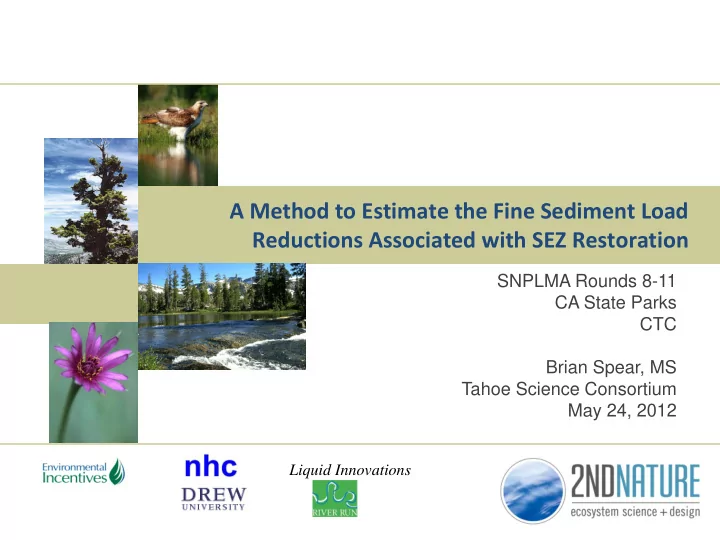
A Method to Estimate the Fine Sediment Load Reductions Associated with SEZ Restoration

SNPLMA Rounds 8-11 CA State Parks CTC Brian Spear, MS Tahoe Science Consortium May 24, 2012

Liquid Innovations

2

Why does Tahoe need load reduction estimates?

• FSP primary pollutant of concern to Lake Tahoe.
• Reduction of FSP loads into Lake Tahoe a priority.

SCG Source Control Treatment Urban Road Abrasives SWT Urban Fertilizer SWT SEZ Channel Erosion Floodplain

3 Southern Pines SEZ Osgood SWT Eloise SWT

Scale = 1:9000

Trout Creek SEZ

SLRT Goal and Objectives

4

• Develop a reliable, repeatable and cost-effective tool
• Applicable to range of SEZ scales
• Incorporates best available data and hypotheses of system

function

• Improvable and adaptable over time
• Consistent with accepted stormwater tools and programs within

Lake Tahoe Basin Method to estimate the average annual pollutant load reduction as a result

• f SEZ restoration actions: Stream Load Reduction Tool (SLRT)

Objectives

5

SEZ Restoration Load Reductions Achieved by: a. Reduce stream bank erosion (source control) b. Increase floodplain deposition (treatment) SLRT Guiding Concepts

6

Users: Practitioners, Engineers, Planners Pollutant: FSP, potential expansion later. Output: Average Annual FSP Load Reduction at downstream boundary of SEZ. EQ1. AA FSP Load Reduction (MT/yr) = AA OUT Pre Restoration (MT/yr) – AA OUT Post Restoration (MT/yr) SLRT Approach

SLRT Approach

7

AA OUT (MT/yr) = IN– SFP + SCE # years

Example Calculation: Trout Creek Restoration Project

8

Load IN= FSP Load Rating Curve x Frequency

9

Time Frame: WY89-WY06

500 1,000 1,500 2,000 2,500

Time (days)

Mean Daily Discharge (cfs)

10336780

0.001 0.01 0.1 1 10 100 1 10 100 1000

FSP Load (MT/day) Mean Daily Discharge (cfs)

Frequency of Occurrence Pollutant Rating Curve

10

Total Load IN = 1,874 MT Load IN = 104 MT/yr Load IN= FSP Load Rating Curve x Frequency

20 40 60 80 100 120 140

Load IN (MT)

Mean Daily Discharge (cfs)

USGS Trout at Pioneer Trail

11

Pre Qcc = 200 cfs Total Load Delivered to FP = 79 MT Retention = Load Delivered to Floodplain x Percent Retained

20 40 60 80 100 120 140

Load Delivered to Floodplain (MT)

Mean Daily Discharge (cfs)

POST pre

Post Qcc = 70 cfs Total Load Delivered to FP = 837 MT

USGS Trout at Pioneer Trail

12

0.00 0.10 0.20 0.30 0.40 0.50 0.60 0.70 0.80 0.90 1.00 0.0 1.0 2.0 3.0 4.0 5.0 6.0

Fraction FSP Retained Discharge: Channel Capacity Ratio

Trout UTR

A B C X Y Z

[FSP] % reduction

longitudinal horizontal interactions

floodplain interaction

Main channel

Retention = Load Delivered x Percent Retained

13

Delivered to Floodplain = 79 MT Retained on Floodplain = 46 MT Pre restoration

10 20 30 40 50 60 70 80 90 100

FSP load (MT)

Mean Daily Discharge (cfs)

PRE DFPfsp PRE SFPfsp

USGS Trout at Pioneer Trail

Qcc = 200 cfs

Retention = Load Delivered x Percent Retained

14

Delivered to Floodplain = 837 MT Retained on Floodplain = 362 MT Post restoration

USGS Trout at Pioneer Trail

10 20 30 40 50 60 70 80 90 100

FSP load (MT)

POST DFPfsp POST SFPfsp

Qcc reduction

Qcc = 70 cfs Qcc = 200 cfs Mean Daily Discharge (cfs)

USGS Trout at Pioneer Trail

Retention = Load Delivered x Percent Retained

Load Reduction of Floodplain Retention

15

Trout Creek Example Summary: Load IN = 104 MT/yr Pre restoration SFP = 2.6 MT/yr Post restoration SFP = 20 MT/yr PRE AA OUT= 101.5 MT/yr POST AA OUT= 84 MT/yr FSP load reduction from FP retention only = 17.5 MT/yr

Next Steps

16

• SCE - collaboration with A. Simon and V. Mahecek to incorporate

BSTEM modeling

• SFP – How can retention coefficient be adjusted for floodplain

characteristics (inundation depth, complexity, vegetation, etc)

• Apply SLRT to urban SEZ project
• Final Technical Report expected Fall 2013
• Data collection summary
• SLRT Technical Document
• SLRT Guidance Document

Summary

17

Plenty of data compilation and analysis

18

• QIN. Complete estimates and then compare to measured datasets.

How well can we predict annual flow volumes? FSP(Q). Compile available data and create best estimations. Document assumptions and provide guidance on how continue in future. Great to get some USGS data.

• Rfsp. Need few more channel/floodplain cross-section morphologies.

Conduct analysis of FP area/depth and veg characteristics Compare site characteristics to Rfsp data obtained. Is Rfsp to Q:Qcc correct or should it be Rfsp to FPz?

• SCE. Coordinate with BSTEM researchers. Develop simple method

and compare results to higher resolution results from Trout and UTR reach.

Stream channel erosion

19

Coordinate with BSTEM researchers. Develop simple method and compare results to higher resolution results from Trout and UTR reach. Critical data gap is the FSP mass per unit of channel sediment generated.

500 1,000 1,500 2,000 2,500

ti (days)

Qmd

AA OUTfsp= (INfsp– SFPfsp + SCEfsp)/18

0.001 0.01 0.1 1 10 100 1 10 100 1000 SCE-FSP (Q) (tons/day) Discharge (cfs)

SLRT calibration using existing datasets

20

Variable Site Duration Calibration approach INfsp Trout at Pioneer Trail WY10/ WY11 Continuous sediment loading data compared to predicted load for spring snow melt events. INfsp Pasadena and Incline urban catchments WY12 Continuous sediment loading data compared to predicted load for events where reliable data is available. SCEfsp Trout from Pioneer Trail to Cold Creek 2002-2006 Compare SLRT simple approach using BSTEM for reduced time series to detailed BSTEM model created for Trout by Simon and Mahacek in late 2009 (SNPLMA). In addition, compare to repeated cross-section dataset to quantify mass of sediment eroded from reach from monitoring points. SCEfsp Bristlecone 1998-2006 Compare SLRT simple approach using BSTEM to results using more rigorous input parameters to evaluate annual deviations and signal in overall OUTfsp load. OUTfsp Trout WY11/WY12 (?) Compare SLRT estimate using event hydrology to measured continuous sediment loading data at Reach 3 boundary.

FSP Data Calculations

21

Post CC (cfs) Pre CC (cfs) ChV post (acft) ChV pre (acft) 70 200 5400 500 ti Post Pre Post Pre Post Pre Post Pre Discharge (cfs) midpoint count FSP(Q) (MT/d) IN fsp(MT) DFPfsp (MT) DFPfsp (MT) Q/Qcc Q/Qcc Rfsp Rfsp SFPfsp SFPfsp 0 To 10 5 2772 0.01 21.77 10 To 20 15 1843 0.06 110.50 m3ps 20 To 30 25 747 0.15 115.23 5.67 30 To 40 35 372 0.29 106.94 2.83 40 To 50 45 229 0.46 104.79 50 To 60 55 125 0.66 82.92 60 To 70 65 90 0.90 81.32 70 To 80 75 69 1.18 81.24 18.90 1.07 0.88 16.7 80 To 90 85 79 1.48 117.25 45.87 1.21 0.76 34.9 90 To 100 95 67 1.82 122.16 61.62 1.36 0.67 41.0 100 To 110 105 52 2.19 114.09 67.11 1.50 0.59 39.6 110 To 120 115 42 2.60 109.04 71.09 1.64 0.53 37.6 120 To 130 125 44 3.03 133.29 93.53 1.79 0.48 44.8 130 To 140 135 33 3.49 115.26 85.45 1.93 0.44 37.3 140 To 150 145 21 3.99 83.72 64.74 2.07 0.40 25.9 150 To 160 155 13 4.51 58.63 46.88 2.21 0.37 17.3 160 To 170 165 6 5.06 30.38 24.96 2.36 0.34 8.6 170 To 180 175 5 5.65 28.23 23.71 2.50 0.32 7.6 180 To 190 185 3 6.26 18.77 16.06 2.64 0.30 4.8 190 To 200 195 2 6.90 13.79 11.99 2.79 0.28 3.4 200 To 210 205 3 7.56 22.69 19.98 2.01 2.93 1.03 0.26 0.93 5.3 1.9 210 To 220 215 5 8.26 41.31 36.79 6.83 3.07 1.08 0.25 0.88 9.2 6.0

Stream FSP Data

22

Stream FSP Data

23

FSP/Turbidity rating curve; cost effective turbidity to FSP by mass conversion

n = 192 OUTfsp= INfsp– SFPfsp + SCEfsp

Stream FSP Data

24

FSP/Q Rating Curves:

• In-Stream

samples

• n = 28

Upper Truckee River OUTfsp= INfsp– SFPfsp + SCEfsp