A Hybrid Monte Carlo Local Branching Algorithm for the Single - PowerPoint PPT Presentation
A Hybrid Monte Carlo Local Branching Algorithm for the Single Vehicle Routing Problem with Stochastic Demands Michel GENDREAU Interuniversity Research Centre on Enterprise Networks, Logistics and Transportation (CIRRELT) Dpartement
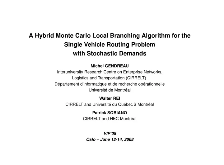
A Hybrid Monte Carlo Local Branching Algorithm for the Single Vehicle Routing Problem with Stochastic Demands Michel GENDREAU Interuniversity Research Centre on Enterprise Networks, Logistics and Transportation (CIRRELT) Département d’informatique et de recherche opérationnelle Université de Montréal Walter REI CIRRELT and Université du Québec à Montréal Patrick SORIANO CIRRELT and HEC Montréal VIP’08 Oslo – June 12-14, 2008
Presentation Outline 1. The single vehicle routing problem with stochastic demands 2. Monte Carlo sampling in stochastic programming 3. Local branching 4. Monte Carlo local branching hybrid algorithm 5. Computational results 6. Conclusion
The Single-Vehicle VRP with Stochastic Demands • A stochastic VRP in which a single capacitated vehicle must deliver (unknown) demands to a set of customers. • Customers demands are revealed only when the vehicle arrives at a given location. • The vehicle follows an a priori (TSP) tour, until it returns to the depot or it cannot meet the demand of a customer (route failure). • When a failure occurs, the vehicle returns to the depot to get replenished (recourse action). • A special case of the classical VRPSD. • More complex recourse strategies (e.g., various restocking schemes) could be handled in the same fashion.
Notation • G ( V, E ) : an undirected graph • V = { v 1 , . . . , v N } : the set of vertices • E = { ( v i , v j ) : v i , v j ∈ V, i < j } : the set of edges • v 1 : the a depot where the vehicle must start and finish its route • ξ j , j ∈ V \ { v 1 } : (stochastic) demand of customer j • D : capacity of the vehicle • C = [ c ij ] : travel costs between vertices N � • f = E [ ξ j ] /D : expected filling rate of the vehicle j =1
Formulation � Min c ij x ij + Q ( x ) (1) i<j N � x 1 j = 2 , s.t. (2) j =2 � x ik + � x kj = 2 , k = 2 , . . . , N, (3) i<k j>k � � x ij + � � x ij ≥ 2 , S ⊆ V, | S | ≥ 3 , (4) i ∈ S j ∈ S, j>i j / ∈ S, j>i i/ ∈ S x ij ∈ { 0 , 1 } , 1 ≤ i < j ≤ N. (5) • Q ( x ) is the recourse function, which gives the expected cost of recourse. • Constraints (2) and (3) ensure that the route starts and ends at the depot and that each customer is visited once. • Inequalities (4) are the subtour elimination constraints.
Previous Work – Exact methods • Gendreau, Laporte, and Séguin (1995): application of 0–1 integer L-shaped algorithm. • Hjorring and Holt (1999): introduction of a new type of cuts that use information taken from partial routes. • Rei, Gendreau, and Soriano (2006): new inequalities based on local branching for the 0–1 integer L-shaped algorithm; excellent results on instances with Normal (independent) demands. Instances where both the filling rate and the number of customers are large still present a tremendous challenge which justifies the development of efficient heuristics for this problem.
Previous Work – Heuristics (Related Problems) • Gendreau, Laporte, and Séguin (1996): tabu search procedure for routing problems where customers and demands are stochastic. • Yang, Mathur, and Ballou (2000): heuristics for routing problems with stochastic demands for which restocking (returning to the depot before visiting the next customer) is consid- ered. • Bianchi et al. (2005): several metaheuristics for stochastic routing problems that allow restocking. • Secomandi (2000, 2001): neuro-dynamic programming algorithms for the case where re- optimization is applied. • Chepuri and Hommem-De-Mello (2005): cross-entropy method to solve an alternate for- mulation (some customers may not be serviced, but at a penalty).
Monte Carlo Sampling in Stochastic Programming Linderoth, Shapiro, and Wright (2006) distinguish two types of approaches: • Interior approaches solve the problem at hand directly, but whenever the algorithm be- ing used requires information concerning the recourse function, sampling is applied to approximate this information. – Dantzig and Glynn (1990): sampling in the L-shaped algorithm to estimate cuts – Higle and Sen (1996): stochastic decomposition – Ermoliev (1988): stochastic quasi-gradient methods (sampling used to produce a quasi- gradient from which a descent direction is obtained) • In the exterior approach, one uses sampling beforehand as a way to approximate the recourse function (next slide).
Sampling the Recourse Function x ∈ X f ( x ) = E ξ [ c ⊤ x + Q ( x, ξ ( ω ))] = c ⊤ x + E ξ [ Q ( x, ξ ( ω ))] . • We want to solve min • Let { ω 1 , . . . , ω n } be a subset of randomly generated events of Ω , then � f n ( x ) = c ⊤ x + n � Q ( x, ξ ( ω i )) is a sample average approximation of f ( x ) . 1 n i =1 � • One may now define the approximating problem as min f n ( x ) . x ∈ X • Mak, Morton, and Wood (1999): the average value of the approximating problem over all possible samples is a lower bound on the optimal value of the problem. � � � • Similarly, if ˜ x is a feasible first-stage solution, then E f n (˜ x ) ≥ f (˜ x ) .
Sampling the Recourse Function (con’d) � � � � � � • By using unbiased estimators for E min f n ( x ) and for E f n (˜ x ) , one can construct con- x ∈ X fidence intervals on the optimal gap associated with ˜ x . • Unbiased estimators can be obtained by using batches of subsets { ω 1 , . . . , ω n } . Let � f j n be the j th sample average approximation function using a randomly generated subset of size m m � � � � v j f j n ( x ) , for j = 1 , . . . , m . Then L n v j n and U n f j 1 1 n and let � n = min m = m = n (˜ x ) � m m x ∈ X j =1 j =1 can be used to estimate the gap associated with ˜ x . � • Under certain conditions, if ˆ x n is an optimal solution to problem min f n ( x ) , then it can be x ∈ X shown that ˆ x n converges with probability 1 to the set of optimal solutions to the original problem as n → ∞ . • Shapiro and Homem-De-Mello (2000): when the probability distribution of ξ is discrete, given some assumptions, ˆ x n is an exact optimal solution for n large enough.
The Sampling Average Approximation Method • Kleywegt, Shapiro, and Homem-De-Mello (2001): definition of the sample average ap- proximation (or SAA) method – Randomly generate batches of samples of random events. – Solve the approximating problems (each solution obtained is an approximation of the optimal solution to the original stochastic problem). – Estimates on the optimal gap using bounds L n m and U n m are then generated to obtain a stopping criterion. – n may be increased if either the gap or the variance of the gap estimation is to large. • The SAA method was adapted for the case of stochastic programs with integer recourse by Ahmed and Shapiro (2002). • Linderoth, Shapiro, and Wright (2006): numerical experiments using the SAA method that show the usefulness of the approach.
Local Branching • A method introduced by Fischetti and Lodi (2003) to take advantage of the fact that certain generic solvers (e.g., CPLEX) are quite efficient to solve small integer 0-1 problems. • Therefore, one can divide the feasible region of a problem into a series of smaller sub- regions and then use a generic solver in order to better explore each of the subregions created. • In the case of a 0-1 integer problem, the function used in order to divide the feasible region is the Hamming distance defined from a given integer point. x ∈ X f ( x ) = c ⊤ x + Q ( x ) , where • Let us suppose that we are solving min – X = { x | Ax = b, x ∈ X ∩ { 0 , 1 } n 1 } , – x 0 is vector of 0-1 values such that x 0 ∈ X , – N 1 = { 1 , . . . , n 1 } and S 0 = { j ∈ N 1 | x 0 j = 1 } , the Hamming distance relative to x 0 is ∆( x, x 0 ) = � � (1 − x j ) + x j . j ∈ S 0 j ∈ N 1 \ S 0
Local Branching (con’d) • Using function ∆( x, x 0 ) , one can divide the feasible region of the problem, by creating two subproblems, one for which the constraint ∆( x, x 0 ) ≤ κ is added, and the other for which ∆( x, x 0 ) ≥ κ + 1 is added (where κ is a certain fixed integer value). • Constraint ∆( x, x 0 ) ≤ κ can considerably reduce the size of the feasible region of problem when value κ is fixed to an appropriate value. • Therefore, one can use an adapted generic solver in order to solve this subproblem. • Using the new solution found, the procedure may continue by dividing the subregion de- fined by ∆( x, x 0 ) ≥ κ + 1 into two more subproblems where the smaller subregion is explored in the same way as before. • If the left the problem is infeasible or unattractive, a diversification procedure is applied (enlarge feasible set).
Monte Carlo Sampling and Local Branching • When using Monte Carlo sampling to approximate the recourse function, one alleviates the stochastic complexity of the problem. • Local branching allows one to control the combinatorial explosion associated with the first- stage of problem. • We now show how principles from Monte Carlo sampling and local branching can be com- bined to form the basis for developing an effective multi-descent heuristic for the SVRPSD.
Local Branching with Sampling A straighforward approach: • Use a fixed-size sample of scenarios to represent demand uncertainty; this defines a simpler SVRPSD, which is just a fairly large MIP . • Solve this MIP with Fischetti and Lodi’s procedure. This is not what we will do.
Recommend
More recommend
Explore More Topics
Stay informed with curated content and fresh updates.

