A history of the k-means algorithm Hans-Hermann Bock, RWTH Aachen, - PowerPoint PPT Presentation

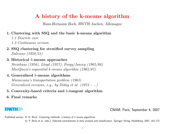
A history of the k-means algorithm Hans-Hermann Bock, RWTH Aachen, Allemagne 1. Clustering with SSQ and the basic k-means algorithm 1.1 Discrete case 1.2 Continuous version 2. SSQ clustering for stratified survey sampling Dalenius (1950/51) 3. Historical k -means approaches Steinhaus (1956), Lloyd (1957), Forgy/Jancey (1965/66) MacQueen’s sequential k -means algorithm (1965/67) 4. Generalized k -means algorithms Maranzana’s transportation problem (1963) Generalized versions, e.g., by Diday et al. (1973 - ...) 5. Convexity-based criteria and k -tangent algorithm 6. Final remarks CNAM, Paris, September 4, 2007 Published version: H.-H. Bock: Clustering methods: a history of k -means algorithms. In: P. Brito et al. (eds.): Selected contributions in data analysis and classification. Springer Verlag, Heidelberg, 2007, 161-172 1

1. Clustering with SSQ and the k -means algorithm Given: O = { 1 , ..., n } set of n objects R p n data vectors x 1 , ..., x n ∈ I Problem: Determine a partition C = ( C 1 , ..., C k ) of O with k classes C i ⊂ O , i = 1 , ..., k characterized by class prototypes: Z = ( z 1 , ..., z k ) Clustering criterion: SSQ, variance criterion, trace criterion, inertie,... k � � || x ℓ − x C i || 2 g ( C ) := → min C i =1 ℓ ∈ C i with class centroids (class means) z ∗ 1 = x C 1 , ..., z ∗ k = x C k . Two-parameter form: k � � || x ℓ − z i || 2 g ( C , Z ) := → min C , Z i =1 ℓ ∈ C i Remark: g ( C ) ≡ g ( C , Z ∗ ) 2

The well-known k -means algorithm C (0) , Z (0) , C (1) , Z (1) ,... • produces a sequence of partitions/prototype systems: t = 0 : Start from an arbitrary initial partition C (0) = ( C (0) 1 , ..., C (0) k ) of O t → t + 1 : (I) Calculate system Z ( t ) of class centroids for C ( t ) : Problem A: � z ( t ) 1 := x C ( t ) = ℓ ∈ C i x ℓ g ( C ( t ) , Z ) → min Z i | C ( t ) i | i (II) Determine the min-dist partition C ( t +1) for Z ( t ) : Problem B: C ( t +1) := { ℓ ∈ O | || x ℓ − z ( t ) i || = min j || x ℓ − z ( t ) j ||} g ( C , Z ( t ) ) → min C i Stopping : Iterate until stationarity, i.e., g ( C ( t ) ) = g ( C ( t +1) ) 3

k � � || x ℓ − z i || 2 g ( C , Z ) := → min C , Z i =1 ℓ ∈ C i Remarks: This two-parameter form contains a continuous ( Z ) and a discrete ( C ) variable. The k -means algorithm is a relaxation algorithm (in the mathematical sense). Theorem: Z ( t ) := Z ( C ( t ) ) The k -means algorithm C ( t +1) := C ( Z ( t ) ) t = 0 , 1 , 2 , ... produces m -partitions C ( t ) and prototype systems Z ( t ) with steadily decreasing criterion values: g ( C ( t ) ) ≡ g ( C ( t ) , Z ( t ) ) ≥ g ( C ( t +1) , Z ( t ) ) ≥ g ( C ( t +1) , Z ( t +1) ) ≡ g ( C ( t +1) ) 4

Continuous version of the SSQ criterion: R p with known distribution P , density f ( x ) Given: A random vector X in I R p R p Problem: Find an ’optimal’ partition B = ( B 1 , ..., B k ) of I I R p , i = 1 , ..., k with k Borel sets (classes) B i ⊂ I characterized by class prototypes: Z = ( z 1 , ..., z k ) • Continuous version of SSQ criterion: � k � || x − E [ X | X ∈ B i ] || 2 dP ( x ) G ( B ) := → min B B i i =1 with class centroids (expectations) z ∗ 1 = E [ X | X ∈ B 1 ] , ..., z ∗ k = E [ X | X ∈ B k ] . • Two-parameter form: � k � || x − z i || 2 dP ( x ) G ( B , Z ) := → min B , Z B i i =1 = ⇒ Continuous version of the k -means algorithm 5

2. Continuous SSQ clustering for stratified sampling Dalenius (1950), Dalenius/Gurney (1951) Given: A random variable (income) X in I R with density f ( x ) σ 2 := V ar ( X ) f ( x ) µ := E [ X ] , Problem: Estimate unknown expected income µ by using n samples (persons) • Strategy I: Simple random sampling Sample n persons, observed income values x 1 , ..., x n � n µ := x = 1 Estimator: ˆ j =1 x j n Performance: E [ˆ µ ] = µ unbiasedness µ ) = σ 2 /n . V ar (ˆ 6

• Strategy II: Stratified sampling Partitioning I R into k classes (strata): B 1 , ..., B k Class probabilities: p 1 , ...., p k f ( x ) Sampling from stratum B i : Y i ∼ X | X ∈ B i B 1 · · · B i · · · B k µ i := E [ Y i ] = E [ X | X ∈ B i ] σ 2 i := V ar ( Y i ) = V ar ( X | X ∈ B i ) ( � k Sampling: n i samples from B i : y i 1 , ..., y in i i =1 n i = n ) � n i µ i := 1 ˆ j =1 y ij n i µ := � k ˆ Estimator: ˆ i =1 p i · ˆ µ i E [ˆ Performance: µ ] = µ (unbiasedness) ˆ � k � p 2 µ ) = � k p i V ar (ˆ · σ 2 ( x − µ i ) 2 dP ( x ) ≤ σ 2 /n i ˆ i = i =1 n i n i B i i =1 • Strategy III: Proportional stratified sampling Use sample sizes proportional to class frequencies: n i = n · p i = ⇒ 7

• Strategy III: Proportional stratified sampling Use sample sizes proportional to class frequencies: n i = n · p i = ⇒ Resulting variance: � � k V ar (ˆ 1 1 B i ( x − µ i ) 2 dP ( x ) = µ ) = ˆ n · G ( B ) → min B i =1 n Implication: Optimum stratification ≡ Optimum SSQ clustering Remark: Dalenius did not use the k -means algorithm for determining B ! 8

3. Les origines: historical k -means approaches • Steinhaus (1956): R p a solid (mechanics; similarly: anthropology, industry) X ⊂ I with mass distribution density f ( x ) X Problem: Dissecting X into k parts B 1 , ..., B k such that sum of class-specific inertias is minimized: � k � || x − E [ X | X ∈ B i ] || 2 f ( x ) dx → min G ( B ) := B B i i =1 Steinhaus proposes: Continuous version of k -means algorithm Steinhaus discusses: – Existence of a solution – Uniqueness of the solution – Asymptotics for k → ∞ 9

• Lloyd (1957): Quantization in information transmission: Pulse-code modulation Problem: Transmitting a p -dimensional random signal X with density f(x) Method: Instead of transmitting the original message (value) x R p – we select k different fixed points (code vectors) z 1 , ..., z k ∈ I – we determine the (index of the) code vector that is closest to x : i ( x ) = argmin j =1 ,...,k {|| x − z j || 2 } – transmit only the index i ( x ) – and decode the message x by the code vector ˆ x := z i ( x ) . Expected transmission (approximation) error: � j =1 ,...,k { || x − z j || 2 } f ( x ) dx = G ( B ( Z ) , Z ) γ ( z 1 , ..., z k ) := min Rp I R p generated by Z = { z 1 , ..., z m } . where B ( Z ) is the minimum-distance partition of I R 1 ) Lloyd’s Method I: Continuous version of k -means (in I 10

• Forgy (1965), Jancey (1966): Taxonomy of genus Phyllota Benth. (Papillionaceae) x 1 , ..., x n are feature vectors characterizing n butterflies Forgy’s lecture proposes the discrete k -means algorithm (implying the SSQ clustering criterion only implicitly!) A strange story: – only indirect communications by Jancey, Anderberg, MacQueen – nevertheless often cited in the data analysis literature 11

Terminology: k -means: – iterated minimum-distance partitioning (Bock 1974) – nu´ ees dynamiques (Diday et al. 1974) – dynamic clusters method (Diday et al. 1973) – nearest centroid sorting (Anderberg 1974) – HMEANS (Sp¨ ath 1975) However: MacQueen (1967) has coined the term ’ k -means algorithm’ for a sequential version: – Processing the data points x s in a sequential order: s=1,2,... – Using the first k data points as ’singleton’ classes (= centroids) – Assigning a new data point x s +1 to the closest class centroid from step s – Updating the corresponding class centroid after the assignment Various authors use ’ k -means’ in this latter (and similar) sense (Chernoff 1970, Sokal 1975) 12

4. La Belle Epoque: Generalized k -means algorithms for clustering criteria of the type: m � � g ( C , Z ) := d ( k, z i ) → min C , Z i =1 k ∈ C i where Z = ( z 1 , ..., z m ) is a system of ’class prototypes’ and d ( k, z i ) = dissimilarity between – the object k (the data point x k ) and – the class C i (the class prototype z i ) Great flexibility in the choice of d and the structure of prototypes z i : – Other metrics than Euclidean metric – Other definitions of a ’class prototype’ (subsets of objects, hyperplanes,...) – Probabilistic clustering models (centroids ↔ m.l. estimation) – New data types: similarity/dissimilarity matrices, symbolic data, ... – Fuzzy clustering 13

• Maranzana (1963): k -means in a graph-theoretical setting Situation: Industrial network with n factories: O = { 1 , ..., n } Pairwise distances d ( ℓ, t ) , e.g., minimum road distance, transportation costs Problem: Transporting commodities from the factories to k suitable warehouses as follows: – Partition O into k classes C 1 , ..., C k – Select, for each class C i , one factory z i ∈ O as ’class-specific warehouse’ (products from a factory ℓ ∈ C i are transported to z i for storing) – Minimize the transportation costs: k � � g ( C , Z ) := d ( ℓ, z i ) → min with z i ∈ C i for i = 1 , ..., m C , Z i =1 ℓ ∈ C i ⇒ k -means-type algorithm : Determining the ’class prototypes’ z i by: � Q ( C i , z ) := d ( ℓ, z ) → min z ∈ C i ℓ ∈ C i Kaufman/Rousseeuw (1987): medoid of C i , partitioning around medoids 14