1 K-means clustering The K-means clustering algorithm can be seen - PDF document

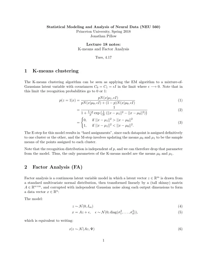
Statistical Modeling and Analysis of Neural Data (NEU 560) Princeton University, Spring 2018 Jonathan Pillow Lecture 18 notes: K-means and Factor Analysis Tues, 4.17 1 K-means clustering The K-means clustering algorithm can be seen as applying the EM algorithm to a mixture-of- Gaussians latent variable with covariances C 0 = C 1 = ǫI in the limit where ǫ − → 0. Note that in this limit the recognition probabilities go to 0 or 1: pN ( x | µ 1 , ǫI ) p ( z = 1 | x ) = (1) pN ( x | µ 0 , ǫI ) + (1 − p ) N ( x | µ 0 , ǫI ) 1 = (2) � 1 2 ǫ ( || x − µ 1 || 2 − || x − µ 0 || 2 ) 1 + 1 − p � p exp � if || x − µ 1 || 2 > || x − µ 0 || 2 0 , = (3) if || x − µ 1 || 2 < || x − µ 0 || 2 . 1 , The E-step for this model results in “hard assignments”, since each datapoint is assigned definitively to one cluster or the other, and the M-step involves updating the means µ 0 and µ 1 to be the sample means of the points assigned to each cluster. Note that the recognition distribution is independent of p , and we can therefore drop that parameter from the model. Thus, the only parameters of the K-means model are the means µ 0 and µ 1 . 2 Factor Analysis (FA) Factor analysis is a continuous latent variable model in which a latent vector z ∈ R m is drawn from a standard multivariate normal distribution, then transformed linearly by a (tall skinny) matrix A ∈ R n × m , and corrupted with independent Gaussian noise along each output dimensions to form a data vector x ∈ R n : The model: z ∼ N (0 , I m ) (4) ǫ ∼ N (0 , diag( σ 2 1 , . . . , σ 2 x = Az + ǫ, d )) , (5) which is equivalent to writing: x | z ∼ N ( Az, Ψ) (6) 1

where I m denotes an m × m identity matrix, and the noise covariance is the diagonal matrix Ψ = diag( σ 2 1 , . . . , σ 2 d ). The model parameters are θ = { A, Ψ } . The columns of the A matrix, which describe how each component of the latent vector affects the output, are called factor loadings . The elements of the i } n diagonal covariance matrix { σ 2 i =1 are known as the uniquenesses . 2.1 Marginal likelihood It is easy to derive the marginal likelihood from the basic Gaussian identities we’ve covered previ- ously, namely: � p ( x | z ) p ( z ) dz = N (0 , AA ⊤ + Ψ) p ( x ) = (7) 3 Identifiability Note the FA model is identifiable only up to a rotation, since if we form ˜ A = AU , where U is A ⊤ = ( AU )( AU ) ⊤ = any m × m orthogonal matrix, then the covariance of the data depends on ˜ A ˜ AUU ⊤ A ⊤ = AA ⊤ . 4 Comparison between FA and PCA FA and PCA are both essentially “just” models of the covariance of the data. The essential difference is that PCA seeks to describe the covariance as low rank (using the m -dimensional subspace that captures the maximal amount of the variance from the d -dimensional response space), whereas FA seeks to describe the covariance as low rank plus a diagonal matrix. FA thus provides a full-rank model of the data, and allows an extra “fudge factor” in the form of (different amounts of) independent Gaussian noise added to the response of each neuron. Thus we can say: • PCA : cov( x ) ≈ USU ⊤ = ( US 1 1 2 )( S 2 U ⊤ ) = BB ⊤ , where U holds the top m eigenvectors of the covariance and S is a diagonal matrix with the m largest eigenvalues of the covariance. • FA : cov( x ) ≈ AA ⊤ + ψ , where AA ⊤ is a rank m matrix that captures shared variability in the responses (which is due to the latent variable), and ψ represents noise to different neurons. PCA is invariant to rotations of the raw data. Running PCA on XU , where U is an n × n orthogonal matrix will return the same principal components (each rotated by U ) and eigenvalues. FA, on the other hand, will change because rotating the data will change shared variance to variance that aligns with the cardinal axes (and vice versa). 2

FA is invariant to independent axis scaling. That is, take measurement x i and multiply it by α . This will change the FA model by scaling the i ’th row of A by α and scaling Ψ ii by α 2 , but the rest of the A and Ψ matrices will remain unchanged. However, scaling an axis can completely change the PCs and their respective eigenvalues. 4.1 Simple example To gain better intuition for the difference between PCA and FA, consider data generated from the FA model with a 1-dimensional latent variable mapping to a 2-neuron population. Let the model parameters be: � 1 � � 100 � 0 A = Ψ = . (8) 1 0 1 Here both neurons load equally onto latent the latent variable (with loading factor 1), but the noise corrupting neuron 1 has 10 times higher standard deviation than the noise corrupting neuron 2. The covariance of the data is therefore: � 101 � 1 cov( x ) = AA ⊤ + Ψ = (9) 1 2 PCA on this model will return a top eigenvector pointing almost entirely along the x 1 axis, since that axis has far more variance than the x 2 axis. The FA model, on the other hand, tells us that the “true” projection of latent into the data space corresponds to a vector along the 45 ◦ diagonal, i.e., the subspace spanned by [1 , 1]. Moreover, the recognition distribution p ( z | x ) will tell us to pay far more attention to x 2 than x 1 for inferring the latent from the neural responses, since x 2 has far less noise. So this corresponds to the orthogonal direction to the PC projection: project onto [01] instead of [10] to get an estimate of z . 3