A differential equation model for multi-class, multi-server queue - PowerPoint PPT Presentation
SANUM Conference March 2016 A differential equation model for multi-class, multi-server queue networks with time dependent parameters. Emma Gibson Prof SE Visagie Operations Research Division, Department of Logistics, Stellenbosch University
SANUM Conference March 2016 A differential equation model for multi-class, multi-server queue networks with time dependent parameters. Emma Gibson Prof SE Visagie Operations Research Division, Department of Logistics, Stellenbosch University
Table of contents 2/33 Introduction 1 Model 2 Queueing theory 3 DE model 4 Results 5 Conclusion 6
Introduction Model Queueing theory DE model Results Conclusion References Zithulele Hospital 3/33
Introduction Model Queueing theory DE model Results Conclusion References Zithulele Hospital 4/33
Introduction Model Queueing theory DE model Results Conclusion References Hospital services 5/33 Nutrition Nutrition Nutrition Nutrition Blood tests X-rays Dental Dental Dental Dental Doctors Doctors Doctors Doctors Doctors Out- Clinics Clinics Clinics Clinics Dispensary Education Education Education Education patients Zithulele Zithulele Zithulele Zithulele Optometry Optometry Optometry Optometry Therapy Hospital Hospital Hospital Hospital In-patients In-patients In-patients Casualty Casualty Maternity Maternity Maternity Surgical Surgical Surgical Fractures Fractures Minor Minor TB TB TB surgery surgery Paediatrics Paediatrics Paediatrics Burns Burns
Introduction Model Queueing theory DE model Results Conclusion References Aims 6/33 Minimise patient waiting times
Introduction Model Queueing theory DE model Results Conclusion References Aims 6/33 Minimise patient waiting times 1. Understand the queueing process: Detailed model Data
Introduction Model Queueing theory DE model Results Conclusion References Aims 6/33 Minimise patient waiting times 1. Understand the queueing process: Detailed model Data 2. Make practical decisions: Ongoing feedback Accessible with matric maths
Introduction Model Queueing theory DE model Results Conclusion References General model 7/33 Clerk Diabetes Vitals TB Triage ARV Blood MVA tests Interaction Patient Xrays Processes Burns profiles Doctor Fractures Pharmacy Certificates Respiratory Dentist Maternity Therapy infections
Introduction Model Queueing theory DE model Results Conclusion References Queueing theory 8/33 Blood Pharmacy Doctor Triage Clerk Vitals X-rays
Introduction Model Queueing theory DE model Results Conclusion References Queueing theory 9/33 q i : number of patients in the i th queue R : routing matrix 4 R 4 , 6 R 2 , 4 R 6 , 7 6 7 R 3 , 4 R 3 , 6 R 1 , 2 R 2 , 3 1 2 3 R 5 , 6 R 3 , 5 5
Introduction Model Queueing theory DE model Results Conclusion References Queueing theory 10/33 λ i : arrival rate µ i : service rate µ i λ i q i
Introduction Model Queueing theory DE model Results Conclusion References Patient profiles 11/33 λ p i : arrival rate for profile p µ p i : service rate for profile p λ 1 µ 1 i i q 1 i . . . . . . . . . q m i λ m µ m i i
Introduction Model Queueing theory DE model Results Conclusion References Problems 12/33 Multi-class queues (Kelly network) Non-stationary arrival rates λ p i ( t ) Time-dependent servers s i ( t ) ∈ N 0 Transient queues - variation in traffic intensity Large state space
Introduction Model Queueing theory DE model Results Conclusion References Fluid approximations 13/33 Deterministic model for expected queue length First-order DE’s Approximate discrete queues with continuous functions Represent arrivals/exits with continuous (mean) flows
Introduction Model Queueing theory DE model Results Conclusion References Equations 14/33 m q p � q i ( t ) = i ( t ) p =1 d q p d t = λ p i ( t ) − µ p i i ( t )
Introduction Model Queueing theory DE model Results Conclusion References Arrival rate 15/33 n λ p i ( t ) = α p � R p j , i µ p i ( t ) + j ( t ) j =1 α p i : external arrival rate for profile p R p j , i : probability of moving from process j → i α p i R p 1 , i µ p 1 . . . λ p µ p i i q p R p j , p µ p j i . . . R p n , i µ p n
Introduction Model Queueing theory DE model Results Conclusion References Traffic intensity 16/33 � m p =1 λ p i ( t ) τ p i ρ i ( t ) = s i ( t ) τ p i : minutes to treat patient type p at process i s i ( t ): staff on duty at process i Case 1: no backlog Case 2: backlog ρ i ( t ) ≤ 1 ρ i ( t ) > 1 and or � m p =1 q p i ( t ) = 0 p =1 q p � m i ( t ) > 0
Introduction Model Queueing theory DE model Results Conclusion References State function 17/33 � p =1 λ p i ( t ) τ p � m 1 i ≤ s i ( t ) && q i ( t ) = 0 φ i ( t ) = 0 otherwise
Introduction Model Queueing theory DE model Results Conclusion References Service rate: no backlog 18/33 Patients are treated on arrival: µ p i ( t ) = λ p i ( t )
Introduction Model Queueing theory DE model Results Conclusion References Service rate: backlog 19/33 New arrivals join the queue. Staff must divide their time between different patient profiles: i ( t ) = β p i ( t ) s i ( t ) µ p τ p i
Introduction Model Queueing theory DE model Results Conclusion References Service rate: backlog 19/33 New arrivals join the queue. Staff must divide their time between different patient profiles: i ( t ) = β p i ( t ) s i ( t ) µ p τ p i Weights β p i are proportional to the number of patients and their treatment needs: β p i ( t ) = c i ( t ) q p i ( t ) τ p i
Introduction Model Queueing theory DE model Results Conclusion References Service rate: backlog 19/33 New arrivals join the queue. Staff must divide their time between different patient profiles: i ( t ) = β p i ( t ) s i ( t ) µ p τ p i Weights β p i are proportional to the number of patients and their treatment needs: β p i ( t ) = c i ( t ) q p i ( t ) τ p i 1 c i ( t ) = � m p =1 q p i ( t ) τ p i
Introduction Model Queueing theory DE model Results Conclusion References Service rate 20/33 s i ( t ) q p i ( t ) µ p i ( t ) = φ i λ p i ( t ) + (1 − φ i ) � m k =1 q k i ( t ) τ k i + φ i � � m p =1 λ p i ( t ) τ p 1 i ≤ s i ( t ) && q i ( t ) = 0 φ i ( t ) = 0 otherwise .
Introduction Model Queueing theory DE model Results Conclusion References Initial DE model 21/33 d q p = λ p i ( t ) − µ p i i ( t ) d t λ p = α p i ( t ) + � n j =1 R p j , i µ p i ( t ) j ( t ) s i ( t ) q p i ( t ) µ p = φ i λ p i ( t ) i ( t ) + (1 − φ i ) � m k =1 q k i ( t ) τ k i + φ i � p =1 λ p i ( t ) τ p � m 1 i ≤ s i ( t ) && q i ( t ) = 0 φ i ( t ) = 0 otherwise .
Introduction Model Queueing theory DE model Results Conclusion References Initial DE model 22/33 Unknown functions: q p i , λ p i , µ p i , φ i Function Units Equation q p Patients Differential i λ p Patients/time Algebraic i µ p Patients/time Algebraic i φ i Binary Algebraic
Introduction Model Queueing theory DE model Results Conclusion References Substitutions 23/33 � t i ( t ) =dΛ p λ p Λ p λ p i i ( t ) = i ( x ) dx d t 0 � t i ( t ) =d U p µ p U p µ p i i ( t ) = i ( x ) dx d t 0
Introduction Model Queueing theory DE model Results Conclusion References Substitutions 24/33 d q p dΛ p d t − d U p i i i d t = d t dΛ p d U p α p i ( t ) + � n j =1 R p i i d t = j , i d t d U p � � d U p s i ( t ) q p i ( t ) α p j =1 R p j i i ( t ) + � n = + (1 − φ i ) φ i j , i � m k =1 q k i ( t ) τ k d t d t i + φ i dΛ p � m d t τ p i 1 i ≤ s i ( t ) && q i ( t ) = 0 k = p φ i ( t ) = 0 otherwise .
Introduction Model Queueing theory DE model Results Conclusion References Substitutions 25/33 q p Λ p i ( t ) − U p i ( t ) = i ( t ) Λ p A p i ( t ) + � n j =1 R p j , i U p i ( t ) = i ( t )
Introduction Model Queueing theory DE model Results Conclusion References Substitutions 26/33 d U p � � d U p s i ( t ) q p i ( t ) j α p i ( t ) + � n j =1 R p i = φ i + (1 − φ i ) j , i � m k =1 q k i ( t ) τ k d t d t i + φ i dΛ p � m i 1 d t τ i ( t ) ≤ s i ( t ) && q i ( t ) = 0 φ i ( t ) = p =1 0 otherwise .
Introduction Model Queueing theory DE model Results Conclusion References Substitutions 26/33 d U p � � d U p s i ( t ) q p i ( t ) j α p i ( t ) + � n j =1 R p i = φ i + (1 − φ i ) j , i � m k =1 q k i ( t ) τ k d t d t i + φ i dΛ p � m i 1 d t τ i ( t ) ≤ s i ( t ) && q i ( t ) = 0 φ i ( t ) = p =1 0 otherwise . q p A p i ( t ) + � n j =1 R p j , i U p i ( t ) − U p i ( t ) → i ( t ) dΛ p d U p α p i ( t ) + � n j =1 R p i i → j , i d t d t
Introduction Model Queueing theory DE model Results Conclusion References Final DE model 27/33 d U p n d U p α p � R p j i = φ i i ( t ) + j , i d t d t j =1 � � A p i ( t ) + � n j =1 R p j , i U p j − U p s i ( t ) i + (1 − φ i ) � � � m i ( t ) + � n k =1 τ k A k j =1 R k j , i U k j − U k + φ i i i d U p � m p =1 ( α p i ( t ) + � n j =1 R p d t ) τ p i 1 i ≤ s i ( t ) j , i A p i ( t ) + � n j =1 R p j , i U p j − U p && i = 0 φ i ( t ) = 0 otherwise .
Recommend
More recommend
Explore More Topics
Stay informed with curated content and fresh updates.
