A Comparison of Imputation Methods under Large Samples and Different - PowerPoint PPT Presentation
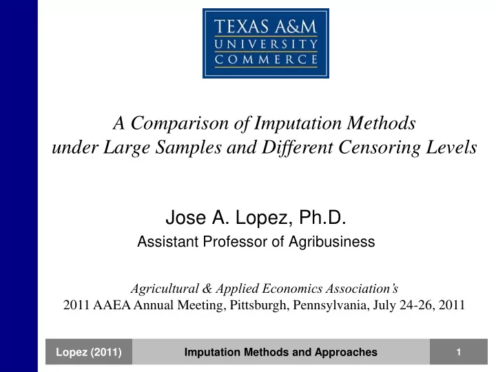
A Comparison of Imputation Methods under Large Samples and Different Censoring Levels Jose A. Lopez, Ph.D. Assistant Professor of Agribusiness Agricultural & Applied Economics Associations 2011 AAEA Annual Meeting, Pittsburgh,
A Comparison of Imputation Methods under Large Samples and Different Censoring Levels Jose A. Lopez, Ph.D. Assistant Professor of Agribusiness Agricultural & Applied Economics Association’s 2011 AAEA Annual Meeting, Pittsburgh, Pennsylvania, July 24-26, 2011 Lopez (2011) Imputation Methods and Approaches 1
Outline 1. Introduction 2. Imputer’s Models 3. Analyst’s Models 4. Data and Procedures 5. Results and Discussion 6. Concluding Remarks Lopez (2011) Imputation Methods and Approaches 2
Introduction • Censored observations – Survey design, implementation, and institutional constrains – Common problem – Usually takes place in high proportions – The value of an observation is partially known (also called item nonresponse) Lopez (2011) Imputation Methods and Approaches 3
Item Nonresponse • Only on the dependent variable – Use of parametric models – The probit and tobit models, or their multinomial versions • Only on an independent variable – Several methods and approaches – Excluding censored observations, deductive imputation, cell mean imputation, hot-deck imputation, cold-deck imputation, complete case analysis, regression imputation, EM algorithm, MCMC algorithm Lopez (2011) Imputation Methods and Approaches 4
Outline 1. Introduction 2. Imputer’s Models 3. Analyst’s Models 4. Data and Procedures 5. Results and Discussion 6. Concluding Remarks Lopez (2011) Imputation Methods and Approaches 5
Excluding Censored Observations • Easy to implement • It discards incompletely recorded units and focuses only on the completely recorded observations (Little and Rubin 2002) – Complete-case analysis • “It can lead to serious bias, however, and it is not usually very efficient, especially when drawing inferences for subpopulations.” (Little and Rubin 2002, p. 19). Lopez (2011) Imputation Methods and Approaches 6
Deductive Imputation • The researcher deduces the missing value by using logic and the relationships among the variables. • If the geographical location of a household is missing, it can be recovered by using other variables such as the consecutive order of household interviews and the time period when the household was interviewed. Lopez (2011) Imputation Methods and Approaches 7
Cell Mean Imputation • Zero-order missing price procedure (Cox and Wolgenant 1986) • Fill-in with means analysis (Little and Rubin 2002) • It consists of grouping the observations (e.g., households) into classes (e.g., strata and state) and using the non-missing values of the variable of interest (e.g., non-missing prices) to impute the missing values of the variable of interest (e.g., missing prices). • The more specific the classes are (e.g., strata and county), the more likely the researcher is to obtain an estimate that is closer to the true value. • The variance in the imputed variable decreases. • To avoid losing variability in the variable of interest, the researcher may alternatively use the mean and standard deviation from the non- missing values of the variable of interest and generate values for imputation from a normal distribution with this mean and this standard deviation. Lopez (2011) Imputation Methods and Approaches 8
Hot Deck Imputation • The term hot deck dates back to the time computer programs and datasets were punched on cards (Lohr1999, p. 275) . • The card reader used to warm the data cards, so the term hot deck was used to refer to the data cards being analyzed. • Similar to cell mean imputation. Lopez (2011) Imputation Methods and Approaches 9
Cold Deck Imputation • It uses a dataset other than the dataset being analyzed to impute the missing value. • These datasets may be from a previous survey or from another source. • Cold deck imputation is common in time series datasets. Lopez (2011) Imputation Methods and Approaches 10
Regression Imputation • Cox and Wohlgenant (1986) – First-order missing price procedure – It combines cell mean imputation with regression imputation • Simple regression imputation Lopez (2011) Imputation Methods and Approaches 11
Cox and Wohlgenant’s (1986) • First, compute the regional mean prices ( mp i ) using the non-missing prices • Second, calculates the corresponding deviations from the regional mean prices ( dmp i ) dpm i = p i – mp i • Third, regresses dmp i as a function household characteristics dpm i = z i ’ β i +e i • Fourth, the missing prices are imputed ^ ~ p dmp mp i i i Lopez (2011) Imputation Methods and Approaches 12
EM Algorithm • The EM algorithm finds the MLE of the vector of parameters by iterating two steps until the iterations converge. • The expectation step (E-step) computes the conditional expectation of the complete-data log likelihood given the observed data and the parameter estimates. Lopez (2011) Imputation Methods and Approaches 13
EM Algorithm (Cont.) • The maximization step (M-step) estimates the parameters that maximize the complete-data log likelihood from the E-step • The observed-data log likelihood being maximized can be expressed as follows G θ θ log ( | ) log ( | ) L X L X • obs g obs 1 g n 1 θ g μ 1 μ • log ( | ) log | | ( )' ( ) L X x x g obs g hg g g hg g 2 2 hg • G = number of groups with distinct missing patterns log L ( θ | X obs ) = the observed-data log likelihood from the g th group • n g = the number of observations in the g th group • The summation is over the household observations in the g th group • • x hg = a vector of observed values corresponding to observed variables • μ g = the mean vector • ∑ g = the associated covariance matrix. Lopez (2011) Imputation Methods and Approaches 14
MCMC Algorithm • The Markov Chain Monte Carlo (MCMC) has applications in Bayesian inference. • This approach consists of a data augmentation procedure that is implemented in two steps. • The imputation step (I-step) draws values for X mis from a conditional predictive distribution of X mis given X obs . • That is, with a current estimate of θ (t) at the t th iteration, θ ( 1 ) θ ( ) t t Pr( | , ) • ~ X X mis obs Lopez (2011) Imputation Methods and Approaches 15
MCMC Algorithm (Cont.) • The posterior step (P-step) draws values for θ from a conditional distribution of θ given X obs θ ( 1 ) θ ( 1 ) t t • ~ Pr | , X X obs mis • The two steps are iterated creating a Markov chain θ θ ( 1 ) ( 1 ) ( 2 ) ( 2 ) , , , , ... • X X mis mis • which converges in distribution to Pr( X mis , θ | X obs ) Lopez (2011) Imputation Methods and Approaches 16
Outline 1. Introduction 2. Imputer’s Models 3. Analyst’s Models 4. Data and Procedures 5. Results and Discussion 6. Concluding Remarks Lopez (2011) Imputation Methods and Approaches 17
Almost Ideal Demand System (AIDS) • The Marshallian demand function for commodity i in share form is specified as m h log( ) log w p • ih i ij jh i ih P j h • w ih = the budget share for commodity i and household h • p jh = the price of commodity j and household h • m h = total household expenditure on the commodities being analyzed • α i , β i and γ ij = parameters • ε i = a random term of disturbances • P h = a price index Lopez (2011) Imputation Methods and Approaches 18
AIDS (Cont.) • In a nonlinear approximation, the price index P h is defined as 1 log( ) log( ) log( ) log( ) P p p p • 0 h k kh kj kh jh 2 k k j • The demand theory properties of adding-up, homogeneity and symmetry can be imposed on the system of equations by restricting parameters in the model as follows 1 , 0 , 0 • Adding-up: i ij i i j i 0 • Homogeneity: ij i • Symmetry: ij ji Lopez (2011) Imputation Methods and Approaches 19
AIDS (Cont.) • The Marshallian (uncompensated) and the Hicksian (compensated) price elasticities as well as the expenditure elasticities can be computed from the estimated coefficients • Marshallian Price Elasticity ij i ln e p ij ij j kj k w w k i i • Hicksian Price Elasticity c e e w e ij ij j i • Expenditure Elasticity 1 i e i w i Lopez (2011) Imputation Methods and Approaches 20
Outline 1. Introduction 2. Imputer’s Models 3. Analyst’s Models 4. Data and Procedures 5. Results and Discussion 6. Concluding Remarks Lopez (2011) Imputation Methods and Approaches 21
Recommend
More recommend
Explore More Topics
Stay informed with curated content and fresh updates.

![Billion Word Imputation Guide: Prof. Amitabha Mukherjee Group 20: Aayush Mudgal [12008] Shruti](https://c.sambuz.com/1085905/billion-word-imputation-s.webp)
