A(b)normal Environments Andrea Condoluci Department of Computer - PowerPoint PPT Presentation
A(b)normal Environments Andrea Condoluci Department of Computer Science and Engineering University of Bologna April 24 th , 2019 Joint work with B. Accattoli, G. Guerrieri & C. Sacerdoti Coen 1/30 A(b)normal Environments Crumbling
A(b)normal Environments Andrea Condoluci Department of Computer Science and Engineering University of Bologna April 24 th , 2019 Joint work with B. Accattoli, G. Guerrieri & C. Sacerdoti Coen 1/30
A(b)normal Environments Crumbling Environments Andrea Condoluci Department of Computer Science and Engineering University of Bologna April 24 th , 2019 Joint work with B. Accattoli, G. Guerrieri & C. Sacerdoti Coen 2/30
Structure of the Presentation Introduction The Curry-Howard-Lambek Correspondence The λ -Calculus Computational Complexity Micro-Step Evaluation Abstract Machines Crumbled Environments A(dministrative) Normal Form Crumbled Terms Crumbling The Crumble GLAM The Machine The Implementation Theorem Complexity Conclusions 3/30
Structure of the Presentation Introduction The Curry-Howard-Lambek Correspondence The λ -Calculus Computational Complexity Micro-Step Evaluation Abstract Machines Crumbled Environments A(dministrative) Normal Form Crumbled Terms Crumbling The Crumble GLAM The Machine The Implementation Theorem Complexity Conclusions 4/30
The Curry-Howard Correspondence (ax) Γ , A ⊢ A Γ , A ⊢ B ( → i) Γ ⊢ A → B Γ ⊢ A → B Γ ⊢ A ( → e) Γ ⊢ B 5/30
The Curry-Howard Correspondence (ax) Γ , x : A ⊢ x : A Γ , x : A ⊢ t : B ( → i) Γ ⊢ λ x . t : A → B Γ ⊢ t : A → B Γ ⊢ u : A ( → e) Γ ⊢ tu : B 5/30
The Curry-Howard Correspondence (ax) Γ , x : A ⊢ x : A Γ , x : A ⊢ t : B ( → i) Γ ⊢ λ x . t : A → B Γ ⊢ t : A → B Γ ⊢ u : A ( → e) Γ ⊢ tu : B ◮ Curry-Howard Correspondence: relationship between mathematical proofs and computer programs ◮ Curry-Howard-Lambek: cartesian closed categories 5/30
The λ -Calculus ◮ At the foundations of OCaml, Haskell, . . . Syntax Terms t , u , s ::= x | λ x . t | t u Examples λ x . x (identity) λ x .λ y . x (1 st projection) 6/30
The λ -Calculus ◮ At the foundations of OCaml, Haskell, . . . Syntax Terms t , u , s ::= x | λ x . t | t u Examples λ x . x (identity) λ x .λ y . x (1 st projection) Evaluation (Top Level) Beta Rule ( λ x . t ) u �→ β t { x � u } Example ( λ x .λ y . x ) t u �→ β ( λ y . t ) u �→ β t . ◮ Reduction → β is the structural closure of �→ β ◮ Evaluation = reducing a λ -term t to its normal form nf( t ) 6/30
Computational Complexity in the λ -calculus ◮ Universal model of computation like Turing machines, Finite state machines, Petri nets, . . . ◮ Church-Turing thesis: computable functions ◮ Computational complexity: classify computational problems according to their inherent difficulty ⇒ How to measure the computational complexity of a λ -term? ◮ Slot and van Emde Boas’ weak invariance thesis: reasonable machines can simulate each other within a polynomial overhead in time ⇒ Is λ -calculus a reasonable machine? 7/30
Size explosion We define the family { t n } n of λ -terms: t 0 := I = λ x . x t n +1 := λ x . t n ( x x ) 8/30
Size explosion We define the family { t n } n of λ -terms: t 0 := I = λ x . x t n +1 := λ x . t n ( x x ) ◮ t 0 = nf( t 0 ) = λ x . x (0 steps) ◮ t 1 = λ x . t 0 ( x x ) = λ x . I ( x x ) → β λ x . x x (1 steps) ◮ t n +1 = λ x . t n ( x x ) → β λ x . ( λ x . x x )( x x ) → β λ x . ( x x )( x x ) 8/30
Size explosion We define the family { t n } n of λ -terms: t 0 := I = λ x . x t n +1 := λ x . t n ( x x ) ◮ t 0 = nf( t 0 ) = λ x . x (0 steps) ◮ t 1 = λ x . t 0 ( x x ) = λ x . I ( x x ) → β λ x . x x (1 steps) ◮ t n +1 = λ x . t n ( x x ) → β λ x . ( λ x . x x )( x x ) → β λ x . ( x x )( x x ) Note that: ◮ | t n | = O ( n ) ◮ t n → n β nf( t n ) ◮ | nf( t n ) | = Ω(2 n ) 8/30
Size explosion We define the family { t n } n of λ -terms: t 0 := I = λ x . x t n +1 := λ x . t n ( x x ) ◮ t 0 = nf( t 0 ) = λ x . x (0 steps) ◮ t 1 = λ x . t 0 ( x x ) = λ x . I ( x x ) → β λ x . x x (1 steps) ◮ t n +1 = λ x . t n ( x x ) → β λ x . ( λ x . x x )( x x ) → β λ x . ( x x )( x x ) Note that: ◮ | t n | = O ( n ) ◮ t n → n β nf( t n ) ◮ | nf( t n ) | = Ω(2 n ) ⇒ Evaluation looks exponential in n and | t | 8/30
Abstract Machines & Complexity ◮ Abstract machines = conceptual models of execution of λ -terms ◮ Enable a quantitative analysis of evaluation: ◮ Bound the asymptotic overhead as a function of the size of the initial term ( | t | ) and the number of β -steps ( n ) ◮ Study the efficiency of abstract machines from a complexity point of view. ◮ First result: Accattoli, Dal Lago (2014) (Leftmost-Outermost) β -Reduction is Invariant, Indeed Efficient machines can reduce λ -terms with only bi-linear overhead, i.e. in time O( | t | · n ). 9/30
Micro-Step Evaluation Computer tools based on the λ -calculus do not implement β -reduction literally. ◮ The substitution t { x � v } performed when firing a redex is not an atomic operation. ◮ If performed without restrictions, it leads to size-explosion (exponential overhead). ◮ Abstract machines employ micro-step evaluation : ◮ The substitutions due to β -steps are delayed and represented as new entries in an environment , and substitution is decomposed as to act on one variable occurrence at a time. 10/30
(Global) Environment Environment : the data structure that stores the delayed substitutions of the previously reduced beta-redexes: term environment ( λ x . t ) u e . . . . . . 11/30
(Global) Environment Environment : the data structure that stores the delayed substitutions of the previously reduced beta-redexes: term environment ( λ x . t ) u e t [ x � u ] e . . . . . . 11/30
(Global) Environment Environment : the data structure that stores the delayed substitutions of the previously reduced beta-redexes: term environment ( λ x . t ) u e t [ x � u ] e . . . . . . Controlled, linear substitution: term environment x [ x � u ] e . . . . . . 11/30
(Global) Environment Environment : the data structure that stores the delayed substitutions of the previously reduced beta-redexes: term environment ( λ x . t ) u e t [ x � u ] e . . . . . . Controlled, linear substitution: term environment x [ x � u ] e u [ x � u ] e . . . . . . 11/30
Dump In abstract machines: search for redexes = “commutative” transition steps. Example The CbV strategy forces the abstract machine to reduce the argument before firing a β -redex. The dump stores the terms to be evaluated next: dump term env ( λ x . t ) u e . . . . . . . . . 12/30
Dump In abstract machines: search for redexes = “commutative” transition steps. Example The CbV strategy forces the abstract machine to reduce the argument before firing a β -redex. The dump stores the terms to be evaluated next: dump term env ( λ x . t ) u e λ x . t u e . . . . . . . . . 12/30
Applicative Stack The applicative stack stores the values that correspond to already evaluated arguments: dump term stack env s u e 13/30
Applicative Stack The applicative stack stores the values that correspond to already evaluated arguments: dump term stack env s u e s u e 13/30
Applicative Stack The applicative stack stores the values that correspond to already evaluated arguments: dump term stack env s u e s u e . . . . . . . . . e ′ s v 13/30
Applicative Stack The applicative stack stores the values that correspond to already evaluated arguments: dump term stack env s u e s u e . . . . . . . . . e ′ s v e ′ - s v 13/30
Applicative Stack The applicative stack stores the values that correspond to already evaluated arguments: dump term stack env s u e s u e . . . . . . . . . e ′ s v e ′ - s v . . . . . . . . . e ′′ λ x . t v 13/30
Applicative Stack The applicative stack stores the values that correspond to already evaluated arguments: dump term stack env s u e s u e . . . . . . . . . e ′ s v e ′ - s v . . . . . . . . . e ′′ λ x . t v [ x � v ] e ′′ t - . . . . . . 13/30
The Open GLAM ◮ Open terms ◮ Global environments ◮ LAM = Leroy Abstract Machine Dump Code Stack Global Env Dump Code Stack Global Env D tu π E � c 1 D : t ♦ π u ǫ E D : t ♦ π λ x . u E D t λ x . u @ ǫ : π E ǫ � c 2 x @ π ′ : π π ′ D : t ♦ π x E � c 3 D t E if E ( x ) = ⊥ D λ x . t φ : π E � m D t π [ x � φ ] E E [ x � φ ] E ′ φ α E [ x � φ ] E ′ D x D π � e π ⇒ Exponential overhead 14/30
The Easy GLAMOUr Optimization: only substitute abstractions, because inert terms do not create new redexes! Dump Code Stack Global Env Dump Code Stack Global Env D tu π E � c 1 D : t ♦ π u ǫ E D : t ♦ π λ x . u ǫ E � c 2 D t λ x . u @ ǫ : π E x @ π ′ : π π ′ D : t ♦ π x E � c 3 D t E if E ( x ) = ⊥ or E ( x ) = y @ π ′′ D λ x . t φ : π E � m D t π [ x � φ ] E E [ x � λ y . u @ ǫ ] E ′ � e λ y . u α E [ x � λ y . u @ ǫ ] E ′ D x D π π 15/30
Recommend
More recommend
Explore More Topics
Stay informed with curated content and fresh updates.
