9.1 Overview 9 Deep Learning Alexander Smola Introduction to - PowerPoint PPT Presentation
9.1 Overview 9 Deep Learning Alexander Smola Introduction to Machine Learning 10-701 http://alex.smola.org/teaching/10-701-15 A brief history of computers 1970s 1980s 1990s 2000s 2010s Data 10 5 10 8 10 2 10 3 10 11 RAM ? 1MB 100MB
9.1 Overview 9 Deep Learning Alexander Smola Introduction to Machine Learning 10-701 http://alex.smola.org/teaching/10-701-15
A brief history of computers 1970s 1980s 1990s 2000s 2010s Data 10 5 10 8 10 2 10 3 10 11 RAM ? 1MB 100MB 10GB 1TB CPU ? 10MF 1GF 100GF 1PF GPU deep kernel deep nets methods nets • Data grows at higher exponent • Moore’s law (silicon) vs. Kryder’s law (disks) • Early algorithms data bound, now CPU/RAM bound
Perceptron x n x 1 x 2 x 3 . . . w n w 1 synaptic weights output y ( x ) = σ ( h w, x i )
Nonlinearities via Layers y 1 i = k ( x i , x ) Kernels y 1 i ( x ) = σ ( h w 1 i , x i ) y 2 ( x ) = σ ( h w 2 , y 1 i ) Deep Nets optimize all weights
Nonlinearities via Layers y 1 i ( x ) = σ ( h w 1 i , x i ) y 2 i ( x ) = σ ( h w 2 i , y 1 i ) y 3 ( x ) = σ ( h w 3 , y 2 i )
Multilayer Perceptron • Layer Representation y y i = W i x i W 4 x i +1 = σ ( y i ) x4 • (typically) iterate between W 3 linear mapping Wx and x3 nonlinear function W 2 • Loss function l ( y, y i ) x2 to measure quality of W 1 estimate so far x1
Backpropagation • Layer Representation y y i = W i x i W 4 x i +1 = σ ( y i ) x4 • Compute change in objective W 3 g j = ∂ W j l ( y, y i ) x3 W 2 • Chain rule x2 ∂ x [ f 2 � f 1 ] ( x ) W 1 = [ ∂ f 1 f 2 � f 1 ( x )] [ ∂ x f 1 ] ( x ) x1
Backpropagation • Layer Representation y y i = W i x i W 4 x i +1 = σ ( y i ) • Gradients x4 ∂ x i y i = W i W 3 ∂ W i y i = x i x3 ∂ y i x i +1 = σ 0 ( y i ) W 2 ⇒ ∂ x i x i +1 = σ 0 ( y i ) W > = i • Backprop x2 W 1 g n = ∂ x n l ( y, y n ) g i = ∂ x i l ( y, y n ) = g i +1 ∂ x i x i +1 x1 ∂ W i l ( y, y n ) = g i +1 σ 0 ( y i ) x > i
Optimization • Layer Representation y y i = W i x i W 4 x i +1 = σ ( y i ) x4 • Gradient descent W 3 W i ← W i − η∂ W i l ( y, y n ) x3 • Second order method W 2 (use higher derivatives) x2 • Stochastic gradient descent W 1 (use only one sample) x1 • Minibatch (small subset)
Things we could learn • Binary classification log(1 + exp( − yy n )) • Multiclass classification (softmax) X exp( y n [ y 0 ]) − y n [ y ] log y 0 • Regression 1 2 k y � y n k 2 • Ranking (top-k) • Preferences • Sequences (see CRFs)
9.2 Layers 9 Deep Learning Alexander Smola Introduction to Machine Learning 10-701 http://alex.smola.org/teaching/10-701-15
Fully Connected • Forward mapping y i = W i x i x i +1 = σ ( y i ) x3 with subsequent nonlinearity W 2 • Backprop gradients x2 ∂ x i x i +1 = σ 0 ( y i ) W > i ∂ W i x i +1 = σ 0 ( y i ) x > i • General purpose layer
Rectified Linear Unit (ReLu) • Forward mapping y i = W i x i x i +1 = σ ( y i ) x3 with subsequent nonlinearity W 2 • Gradients vanish at tails x2 • Solution - replace by max(0,x) • Derivative is in {0; 1} • Sparsity of signal (Nair & Hinton, machinelearning.wustl.edu/mlpapers/paper_files/icml2010_NairH10.pdf)
Where is Wally
LeNet for OCR (1990s)
Convolutional Layers • Images have translation invariance (to some extent) • Low level is mostly edge and feature detectors • Usually via convolution (plus nonlinearity)
Convolutional Layers • Images have translation invariance • Forward (usually implemented brute force) y i = x i � W i x i +1 = σ ( y i ) • Backward gradients (need to convolve appropriately)
Subsampling & MaxPooling • Multiple convolutions blow up dimensionality • Subsampling - average over patches (this works decently) • MaxPooling - pick the maximum over patches (often non overlapping ones)
Depth vs. Width • Longer range effects • many narrow convolutions • few wide convolutions • More nonlinearities work better (same number of parameters) Simonyan and Zisserman arxiv.org/pdf/1409.1556v6.pdf
Fancy structures • Compute different filters • Compose one big vector from all of them • Layer this iteratively Szegedy et al. arxiv.org/pdf/1409.4842v1.pdf
Whole system training Le Cun, Bottou, Bengio, Haffner, 2001 yann.lecun.com/exdb/publis/pdf/lecun-01a.pdf
Whole system training • Layers need not be ‘neural networks’ • Rankers • Segmenters • Finite state automata • Jointly train a full OCR system Le Cun, Bottou, Bengio, Haffner, 2001 yann.lecun.com/exdb/publis/pdf/lecun-01a.pdf
9.3 Objectives 9 Deep Learning Alexander Smola Introduction to Machine Learning 10-701 http://alex.smola.org/teaching/10-701-15
Classification • Binary classification log(1 + exp( − yy n )) Binary exponential model • Multiclass classification (softmax) Multinomial exponential model e y n [ y ] e y n [ y 0 ] − y n [ y ] X − log p ( y | y n ) = − log y 0 e y n [ y 0 ] = log P y 0 • Pretty much anything else we did so far in 10-701
Regression • Least mean squares 1 2 k y � y n k 2 2 this works for vectors, too • Applications • Stock market prediction (more on this later) • Image superresolution (regress from lower dimensional to higher dimensional image) • Recommendation and rating (Netflix)
Autoencoder • Regress from observation to itself (y n = x 1 ) • Lower-dimensional layer x1 is bottleneck V 1 • Often trained iteratively x2 x1 V 1 V 2 x2 x3 W 1 W 2 x1 x2 W 1 x1
Autoencoder • Regress from observation to itself (y n = x 1 ) • Lower-dimensional layer x1 is bottleneck V 1 • Often trained iteratively x2 • Extracts approximate V 2 sufficient statistic of data x3 W 2 • Special case - PCA x2 • linear mapping W 1 • only single layer x1
‘Synesthesia’ • Different data sources • Images and captions • Natural language queries and SQL queries • Movies and actions • Generative embedding for both entities • Minimize distance between pairs • Need to prevent clumping all together
‘Synesthesia’ • Different data sources • Images and captions • Natural language queries and SQL queries • Movies and actions max(0 , margin + d ( a, b ) − d ( a, n )) large margin of similarity Grefenstette et al, 2014, arxiv.org/abs/1404.7296
Synthetic Data Generation • Dataset often has useful invariance • Images can be shifted, scaled, RGB transformed, blurred, sharpened, etc. • Speech can have echo, background noise, environmental noise • Text can have typos, omissions, etc. • Generate data and train on extended noisy set • Record breaking speech recognition (Baidu) • Record breaking image recognition (Baidu, LeCun) • Can be very computationally expensive
Synthetic Data Generation • Sample according to relevance of transform • Similar to Virtual Support Vectors (Schölkopf, 1998) • Training with input noise & regularization (Bishop, 1995)
9.4 Optimization 9 Deep Learning Alexander Smola Introduction to Machine Learning 10-701 http://alex.smola.org/teaching/10-701-15
Stochastic Gradient Descent • Update parameters according to W ij ← W ij − η ij ( t ) g ij • Rate of decay • Adjust each layer • Adjust each parameter individually • Minibatch size • Momentum terms • Lots of things that can (should) be adjusted (via Bayesian optimization, e.g. Spearmint, MOE) Senior, Heigold, Ranzato and Yang, 2013 http://static.googleusercontent.com/media/research.google.com/en/us/pubs/archive/40808.pdf
Minibatch • Update parameters according to W ij ← W ij − η ij ( t ) g ij • Aggregate gradients before applying • Reduces variance in gradients • Better for vectorization (GPUs) vector, vector < vector, matrix < matrix, matrix • Large minibatch may need large memory (and slow updates). • Magic numbers are 64 to 256 on GPUs Senior, Heigold, Ranzato and Yang, 2013 http://static.googleusercontent.com/media/research.google.com/en/us/pubs/archive/40808.pdf
Learning rate decay • Constant (requires schedule for piecewise constant, tricky) • Polynomial decay α η ( t ) = ( β + t ) γ Recall exponent of 0.5 for conventional SGD, 1 for strong convexity. Bottou picks 0.75 • Exponential decay η ( t ) = α e − β t risky since decay could be to aggressive
AdaGrad • Adaptive learning rate (preconditioner) η 0 η ij ( t ) = q t g 2 K + P ij ( t ) • For directions with large gradient, decrease learning rate aggressively to avoid instability • If gradients start vanishing, learning rate decrease reduces, too • Local variant η t η ij ( t ) = q K + P t t 0 = t � τ g 2 ij ( t 0 ) Duchi, Hazan, Singer, 2010 http://www.magicbroom.info/Papers/DuchiHaSi10.pdf
Momentum • Average over recent gradients • Helps with local minima momentum • Flat (noisy) gradients m t = (1 − λ ) m t − 1 + λ g t w t ← w t − η t g t − ˜ η t m t • Can lead to oscillations for large momentum • Nesterov’s accelerated gradient m t +1 = µm t + ✏ g ( w t − µm t ) w t +1 = w t − m t +1
Recommend


More recommend
Explore More Topics
Stay informed with curated content and fresh updates.