5.1 Online versus Offline SVMs We start with a review of the - PDF document

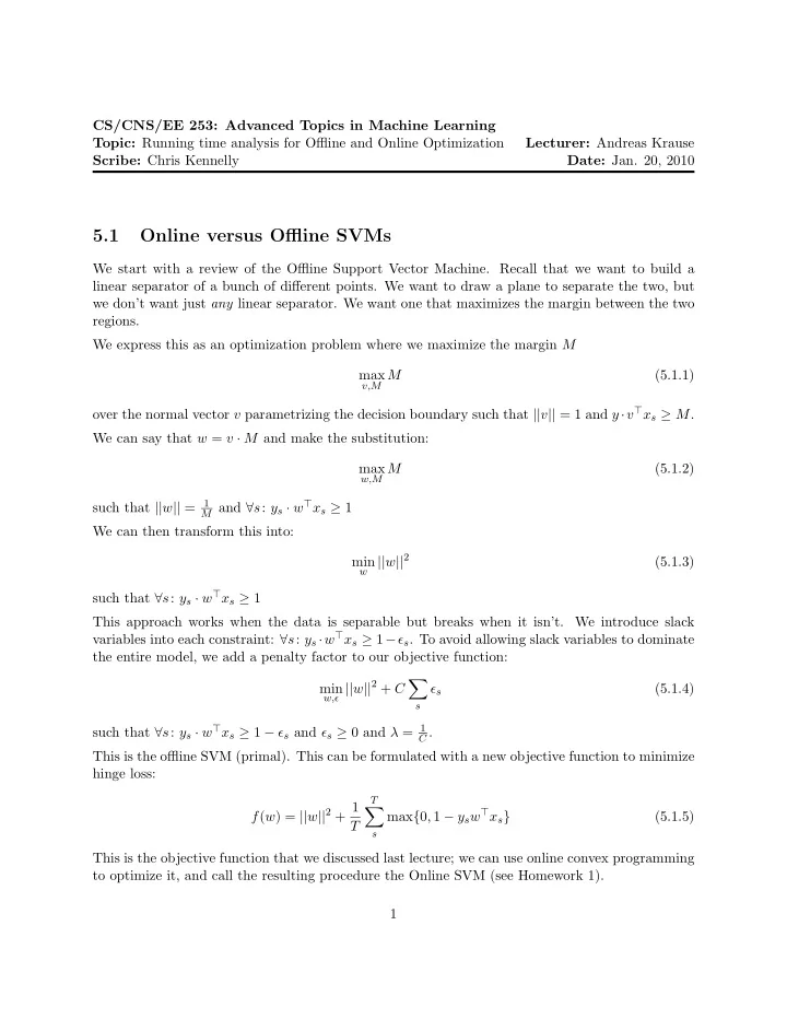
CS/CNS/EE 253: Advanced Topics in Machine Learning Topic: Running time analysis for Offline and Online Optimization Lecturer: Andreas Krause Scribe: Chris Kennelly Date: Jan. 20, 2010 5.1 Online versus Offline SVMs We start with a review of the Offline Support Vector Machine. Recall that we want to build a linear separator of a bunch of different points. We want to draw a plane to separate the two, but we don’t want just any linear separator. We want one that maximizes the margin between the two regions. We express this as an optimization problem where we maximize the margin M max (5.1.1) v,M M over the normal vector v parametrizing the decision boundary such that || v || = 1 and y · v ⊤ x s ≥ M . We can say that w = v · M and make the substitution: max w,M M (5.1.2) 1 M and ∀ s : y s · w ⊤ x s ≥ 1 such that || w || = We can then transform this into: w || w || 2 min (5.1.3) such that ∀ s : y s · w ⊤ x s ≥ 1 This approach works when the data is separable but breaks when it isn’t. We introduce slack variables into each constraint: ∀ s : y s · w ⊤ x s ≥ 1 − ǫ s . To avoid allowing slack variables to dominate the entire model, we add a penalty factor to our objective function: � w,ǫ || w || 2 + C min ǫ s (5.1.4) s such that ∀ s : y s · w ⊤ x s ≥ 1 − ǫ s and ǫ s ≥ 0 and λ = 1 C . This is the offline SVM (primal). This can be formulated with a new objective function to minimize hinge loss: T f ( w ) = || w || 2 + 1 � max { 0 , 1 − y s w ⊤ x s } (5.1.5) T s This is the objective function that we discussed last lecture; we can use online convex programming to optimize it, and call the resulting procedure the Online SVM (see Homework 1). 1

5.1.1 Running-time Analysis How does this approach scale with dataset size? Typically, we take an algorithm, give it a dataset, and measure how long it takes. Generally, we would expect the running time to increase with data set size. In this lecture, we will, perhaps counterintuitively, see that in learning, running time can decrease with data set size. In learning, we want to minimize the objective function. Most of the algorithms are iterative in nature and will–hopefully–converge to the optimal value. We can set a goal for a particular target error ǫ and stop early when we achieve it – thus, we may not have to process the entire data set. If I fix a bound ǫ on the error, what is my running time to achieve this error? If I consider a fresh data point at every iteration, I should eventually reach an error level ǫ after a number of iterations and not see significant improvement even if my dataset increases in size . How many iterations do I need to get a small training error? In an offline setting, the entire training set can be examined to measure error expressed by f ( ˜ w ) ≤ min w f ( w ) + ǫ acc , where ǫ acc is a bound on the approximation accuracy (that we allow ourselves when running the optimization procedure). There are a number of techniques to perform this optimization. 1 • Sequential minimum optimization (SMO)–a commonly technique–requires log ǫ acc iterations at a cost of m 2 per iteration (where m is the size of the training set). ǫ acc iterations at a cost of m 3 . 5 per iteration. 1 • Interior point methods require log log For online settings, 1 • The algorithm discussed in class gives an algorithm requiring ǫ 2 iterations, with constant √ cost per iteration 1 • The version in the Homework (called PEGASOS) improves that to λǫ iterations, again with constant cost per iteration The online techniques have substantially lower costs per iteration at the expense of slower conver- gence rates. Armed with a million data points, these offline techniques become very computationally expensive. When is the break-even point between the algorithms? The key idea is to not look at the training set error, but the generalization error (i.e., expected error on test set). 2

5.2 Generalization Consider m f ( w ) = f λ ( w ) = λ || w || 2 + 1 � l ( w i ( x i , y i )) m i =1 The training set is sampled i.i.d. from the data set. Suppose ( x i , y i ) ∼ P . So the expected error of w is l ( w ) = E ( x,y ) ∼ D l ( w i ( x, y )). Ideally, we’d like to find w ∗ = arg min l ( w ). One approach would be to use empirical risk minimization ˆ w E = arg min l ( w ) , W � m where ˆ l ( w ) = 1 i =1 l ( w i ( x i , y i )). m Because of the law of large numbers, as we obtain more and more examples, ˆ l converges to l . Unfortunately, for small m , the variance of this estimator will be very large, and we will overfit. Instead, we use Regularized risk minimization : w λ = arg min w f λ ( w ) λ controls the trade-off between “goodness of fit” and model complexity. Define w ∗ λ = arg min w E [ f λ ( w )] As we obtain more data, l ( w ∗ λ ) is fixed. l ( w λ ) will be worse than l ( w ∗ λ ) as it is based only on the data we have, but will converge to l ( w ∗ λ ) as more data is received. This gives three sources of error: • Approximation error: l ( w ∗ λ ), due to regularization ( λ > 0, i.e., we’re not minimizing the true loss l but f λ ). • Estimation error: l ( w λ ) − l ( w ∗ λ ), due to our limitations in being able to estimate error from limited data • Training error: l ( ˜ w ) − l ( w λ ), due to running our optimization algorithm for a finite number of iterations (i.e., ǫ acc > 0). We want to ensure our generalization error is at most ǫ . We can vary our model λ and ǫ acc to reach that goal. As we get more and more data, we can be “sloppy” as our estimation error is sufficiently low. Even given unbounded running time, we may have too little data to obtain a desired ǫ ; this is called the “data bounded regime.” 3

Contrast the data bounded regime with the hypothetical scenerio of infinite data. Suppose ∃ w 0 , a 1 hyperplane with large margin M = || w 0 || and low loss l ( w 0 ). This hyperplane will be optimal and we will attempt to approximate it by ˜ w : � || w 0 || 2 − || ˜ w || 2 � l ( ˜ w ) = l ( w 0 ) + λ + E [ f ( ˜ w ) − f ( w 0 )] Since this will be used to adjust how far we go in our optimization, we want to rewrite this equation in terms of otpimization error. Theorem 5.2.1 With probability ≥ 1 − δ : ≤ ǫ acc � �� � +log 1 � � ˆ w ) ≤ l ( w 0 ) + λ || w 0 || 2 + δ l ( ˜ 2 f ( ˜ w ) − f ( w 0 ) λm We want | f ( ˜ w ) − f ( w 0 ) | < ǫ . We can choose λ, ǫ acc , m so that each component of error is bounded by 1 3 ǫ . This gives the relations � � ǫ λ = O || w 0 || 2 = O ( ǫ ) ǫ acc � || w ∗ � 0 || 2 m = Ω ǫ 2 If we have larger margins, we need fewer data points. If we want lower error, we need more data points. 5.2.1 Finite Data In practice, we don’t have infinite data. m is ultimately bounded. This constrains our choices for the other constants. For an online SVM (PEGASOS): w ) ≤ l ( w 0 ) + O ( 1 λT ) + λ || w 0 || 2 + O ( 1 l ( ˜ λm ) � √ 1 /T + √ � 1 /m Minimizing for λ , we pick λ = θ . || w 0 || This gives running time as a function of m and ǫ : � � 1 T ( m ; ǫ ) = θ || w 0 || − O ( 1 ǫ √ m ) 2 Further analysis shows that there is some minimal running time due to our error. Additionally, if there is too little data, we can run our algorithm for as long as we like and never obtain our desired generalization error. If we have more data, we can get our algorithm to unexpectedly run faster . 4