4. Source Encoding Methods Called also entropy coders , because the - PowerPoint PPT Presentation

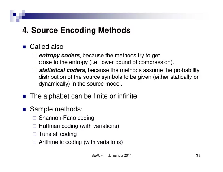
4. Source Encoding Methods � Called also � entropy coders , because the methods try to get close to the entropy (i.e. lower bound of compression). � statistical coders , because the methods assume the probability distribution of the source symbols to be given (either statically or dynamically) in the source model. � The alphabet can be finite or infinite � Sample methods: � Shannon-Fano coding � Huffman coding (with variations) � Tunstall coding � Arithmetic coding (with variations) SEAC-4 J.Teuhola 2014 38

4.1. Shannon-Fano code � First idea: Code length l i = ⎡ log 2 p i ⎤ . � This satisfies: H ( S ) ≤ L ≤ H ( S ) + 1 � Always possible, because Kraft inequality is satisfied: 1 1 ∑ ∑ ∑ ≥ ⇒ ≥ ⇒ ≥ ⇒ ≥ l l log 2 ( 1 / p ) p 1 / 2 p 1 i i i i i l l 2 2 i i Problems: � The decoding tree may not be complete (succinct). � How to assign codewords? � Shannon-Fano method solves these problems by balanced top-down decomposition of the alphabet. SEAC-4 J.Teuhola 2014 39

Example � p 1 = p 2 = 0.3: code lengths: ⎡− log 2 0.3 ⎤ = 2 � p 3 = p 4 = p 5 = p 6 = 0.1: code lengths: ⎡− log 2 0.1 ⎤ = 4 � E.g. 1 0 0 1 0 1 0 1 s 1 s 2 ? 0 1 0 1 s 3 s 4 s 5 s 6 SEAC-4 J.Teuhola 2014 40

Algorithm 4.1. Shannon-Fano codebook generation Input : Alphabet S = { s 1 , ..., s q }, probability distribution P = { p 1 , ..., p q }, where p i ≥ p i +1. Output : Decoding tree for S . begin Create a root vertex r and associate alphabet S with it. If S has only one symbol then return r . ∑ = ∑ j q Find j ( ≠ 0 and ≠ q ) such that p and are p i = + i i 1 i j 1 the closest. Find decoding trees r 1 and r 2 for the sub-alphabets { s 1 , ..., s j } and { s j +1, ..., s q } recursively and set them to subtrees of r , with labels 0 and 1. Return the tree rooted by r . end SEAC-4 J.Teuhola 2014 41

(1) (2) (3) {a,b,c,d,e,f}: 1.0 {a,b,c,d,e,f}: 1.0 {a,b,c,d,e,f}: 1.0 0 1 0 1 {a,b}: 0.6 {c,d,e,f}: 0.4 0 1 {a,b}: 0.6 {c,d,e,f}: 0.4 a: 0.3 b: 0.3 (4) (5) {a,b,c,d,e,f}: 1.0 {a,b,c,d,e,f}: 1.0 0 1 0 1 {c,d,e,f}: 0.4 {c,d,e,f}: 0.4 {a,b}: 0.6 {a,b}: 0.6 0 1 0 1 0 1 0 1 {c,d} {e,f}: 0.2 0.2 0 1 0 1 b: 0.3 {c,d}: 0.2 {e,f}: 0.2 a:0.3 b:0.3 a: 0.3 c:0.1 d:0.1 e:0.1 f:0.1 SEAC-4 J.Teuhola 2014 42

4.2. Huffman code Best-known source compression method. � Builds the tree bottom-up (contrary to Shannon-Fano). � Principles: Two least probable symbols appear as lowest-level � leaves in the tree, and differ only at the last bit. A pair of symbols s i and s j can be considered a meta- � symbol with probability p i + p i . Pairwise combining is repeated q -1 times. � SEAC-4 J.Teuhola 2014 43

Algorithm 4.2. Huffman codebook generation Input : Alphabet S = { s 1 , ..., s q }, probability distribution P = { p 1 , ..., p q }, where p i ≥ p i +1 . Output : Decoding tree for S . begin Initialize forest F to contain a one-node tree T i for each symbol s i and set weight ( T i ) = p i . while | F | > 1 do begin Let X and Y be two trees with the lowest weights. Create a binary tree Z , with X and Y as subtrees (equipped with labels 0 and 1). Set weight ( Z ) = weight ( X ) + weight ( Y ). Add Z to forest F and remove X and Y from it. end Return the single remaining tree of forest F . end SEAC-4 J.Teuhola 2014 44

Example of Huffman codebook generation (1) (2) 0.2 0 1 0.3 0.3 0.1 0.1 0.1 0.1 0.3 0.3 0.1 0.1 0.1 0.1 a b c d e f a b c d e f (3) (4) 0 0.4 1 0.2 0.2 0.2 0.2 0 1 0 1 0 1 0 1 0.3 0.3 0.1 0.1 0.1 0.1 0.3 0.3 0.1 0.1 0.1 0.1 a b c d e f a b c d e f (5) (6) 0 1.0 1 0.4 0 0.4 0 1 1 0.2 0.6 0.2 0.2 0.6 0.2 0 1 0 1 0 1 0 1 0 1 0 1 0.3 0.3 0.1 0.1 0.1 0.1 0.3 0.3 0.1 0.1 0.1 0.1 a b c d e f a b c d e f SEAC-4 J.Teuhola 2014 45

Properties of Huffman code � Produces an optimal codebook for the alphabet, assuming that the symbols are independent. � The average code length reaches the lower bound (entropy) if p i = 2 -k where k is an integer. � Generally: H ( S ) ≤ L ≤ H(S)+p 1 +0.086, where p 1 is the largest symbol probability. � The codebook is not unique: (1) Equal probabilities can be combined using any tie-break rule. (2) Bits 0 and 1 can be assigned to subtrees in either order. SEAC-4 J.Teuhola 2014 46

Implementation alternatives of Huffman code 1. Maintain a min-heap , ordered by weight; the smallest can be extracted from the root. The complexity of building the tree: O ( q ), inserting a metasymbol: O (log q ); altogether O ( q log q ). 2. Keep the uncombined symbols in a list sorted by weight, and maintain a queue of metasymbols. � The two smallest weights can be found from these two sequences � The new (combined) metasymbol has weight higher than the earlier ones. � Complexity: O ( q ), if the alphabet is already sorted by probability. SEAC-4 J.Teuhola 2014 47

Special distributions for Huffman code � All symbols equally probable, q = 2 k , where k is integer: block code . � All symbols equally probable, no k such that q = 2 k : shortened block code . � Sum of two smallest probabilities > largest: (shortened) block code. � Negative exponential distribution: p i = c · 2 - i : codewords 0, 10, 110 , ..., 111..10, 111..11 (cf. unary code). � Zipf distribution : p i ≈ c / i (symbols s i sorted by probability): compresses to about 5 bits per character for normal text. SEAC-4 J.Teuhola 2014 48

Transmission of the codebook � Drawback of (static) Huffman coding: The codebook must be stored/transmitted to the decoder � Alternatives: � Shape of the tree (2 q -1 bits) plus leaf symbols from left to right ( q ⎡ log 2 q ⎤ bits). � Lengths of codewords in alphabetic order (using e.g. universal coding of integers); worst case O( q log 2 q ) bits. � Counts of different lengths, plus symbols in probability order; space complexity also O( q log 2 q ) bits. SEAC-4 J.Teuhola 2014 49

Extended Huffman code Huffman coding does not work well for: Small alphabet � Skew distribution � Entropy close to 0, average code length yet ≥ 1. � Solution: Extend the alphabet to S ( n ): � Take n -grams of symbols as units in coding. Effect: larger alphabet ( q n ), decreases the largest � probability. SEAC-4 J.Teuhola 2014 50

Extended Huffman code (cont.) � Information theory gives: H ( S(n) ) ≤ L(n) ≤ H ( S(n) ) + 1 � Counted per original symbol: H ( S(n) )/ n ≤ L ≤ ( H ( S(n) ) + 1)/ n which gives (by independence assumption): H ( S ) ≤ L ≤ H ( S ) + 1/ n � Thus : Average codeword length approaches the entropy. � But: The alphabet size grows exponentially, most of the extended symbols do not appear in messages for large n . � Goal: No explicit tree; codes determined on the fly. SEAC-4 J.Teuhola 2014 51

Adaptive Huffman coding Normal Huffman coding : Two phases, static tree � Adaptive compression: The model (& probability � distribution) changes after each symbol; encoder and decoder change their models intact. Naive adaptation: Build a new Huffman tree after each � transmitted symbol, using the current frequencies. Observation: The structure of the tree changes rather � seldom during the evolution of frequencies. Goal: Determine conditions for changing the tree, and � the technique to do it. SEAC-4 J.Teuhola 2014 52

Adaptive Huffman coding (cont.) � Sibling property: Each node, except the root, has a sibling (i.e. the binary tree is complete). � The tree nodes can be listed in non-decreasing order of weight so that each node is adjacent in the list to its sibling. � Theorem. A binary tree having weights associated with its nodes, as defined above, is a Huffman tree if and only if it has the sibling property. Proof. Skipped. SEAC-4 J.Teuhola 2014 53

Implementation of Adaptive Huffman coding � Start from a balanced tree with weight = 1 for each leaf; the weight of an internal node = sum of child weights. � Maintain a threaded list of tree nodes in increasing order of weight. � Nodes of equal weight in the list form a (virtual) block . � After transmitting the next symbol, add one to the weights of nodes on the path from the correct leaf up to the root. � Increasing a node weight by one may violate the increasing order within the list. � Swapping of violating node with the rightmost node in the same block will recover the order, and maintains the sibling property. Addition of frequencies continues from the new parent. SEAC-4 J.Teuhola 2014 54

Example of Huffman tree evolution Increase the weight of ’a’ from 1 to 2: r 10 9 r w x 4 6 6 w 3 y 3 x 3 z 3 3 2 2 y z a b 2 1 a b SEAC-4 J.Teuhola 2014 55

Example step in adaptive Huffman coding 9 r r 6 w 3 y 10 3 3 6 4 w x x z 1 2 3 3 2 2 y z a b a b SEAC-4 J.Teuhola 2014 56

Notes about Adaptive Huffman coding Modification: � Start from an empty alphabet, and a tree with only a placeholder . � At the first occurrence of a symbol, transmit the placeholder code and symbol as such, insert it to the tree by splitting the placeholder node. Further notes: � Complexity proportional to the number of output bits. � Compression power close to static Huffman code. � Not very flexible in context-dependent modelling. SEAC-4 J.Teuhola 2014 57