Compression Programs File Compression: Gzip, Bzip Archivers :Arc, - PDF document
Analysis of Algorithms Analysis of Algorithms Analysis of Algorithms Piyush Piyush Kumar Kumar (Lecture 4: Compres (Lect (Lect (Lecture 4: Compres e 4: Compression e 4: Compression on) on) Welcome to 4531 Source: Guy E. Blelloch,
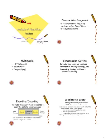
Analysis of Algorithms Analysis of Algorithms Analysis of Algorithms Piyush Piyush Kumar Kumar (Lecture 4: Compres (Lect (Lect (Lecture 4: Compres e 4: Compression e 4: Compression on) on) Welcome to 4531 Source: Guy E. Blelloch, Emad, Tseng … Compression Programs • File Compression: Gzip, Bzip • Archivers :Arc, Pkzip, Winrar, … • File Systems: NTFS Multimedia • HDTV (Mpeg 4) • Sound (Mp3) • Images (Jpeg) 1
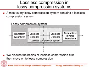
Compression Outline Introduction : Lossy vs. Lossless Information Theory : Entropy, etc. Probability Coding : Huffman + Arithmetic Coding Encoding/Decoding Will use “message” in generic sense to mean the data to be compressed Input Compressed Output Encoder Decoder Message Message Message CODEC The encoder and decoder need to understand common compressed format. Lossless vs. Lossy Lossless : Input message = Output message Lossy : Input message ≈ Output message Lossy does not necessarily mean loss of quality. In fact the output could be “better” than the input. – Drop random noise in images (dust on lens) – Drop background in music – Fix spelling errors in text. Put into better form. Writing is the art of lossy text compression. 2
Lossless Compression Techniques • LZW (Lempel-Ziv-Welch) compression – Build dictionary – Replace patterns with index of dict. • Burrows-Wheeler transform – Block sort data to improve compression • Run length encoding – Find & compress repetitive sequences • Huffman code – Use variable length codes based on frequency How much can we compress? For lossless compression, assuming all input messages are valid, if even one string is compressed, some other must expand. Model vs. Coder To compress we need a bias on the probability of messages. The model determines this bias Encoder Messages Probs. Bits Model Coder Example models: – Simple: Character counts, repeated strings – Complex: Models of a human face 3
Quality of Compression Runtime vs. Compression vs. Generality Several standard corpuses to compare algorithms Calgary Corpus • 2 books, 5 papers, 1 bibliography, 1 collection of news articles, 3 programs, 1 terminal session, 2 object files, 1 geophysical data, 1 bitmap bw image The Archive Comparison Test maintains a comparison of just about all algorithms publicly available Comparison of Algorithms Program Algorithm Time BPC Score BOA PPM Var. 94+97 1.91 407 PPMD PPM 11+20 2.07 265 IMP BW 10+3 2.14 254 BZIP BW 20+6 2.19 273 GZIP LZ77 Var. 19+5 2.59 318 LZ77 LZ77 ? 3.94 ? Information Theory An interface between modeling and coding • Entropy – A measure of information content • Entropy of the English Language – How much information does each character in “typical” English text contain? 4
Entropy (Shannon 1948) For a set of messages S with probability p(s), s ∈ S , the self information of s is: 1 = = − i s ( ) log log ( ) p s p s ( ) Measured in bits if the log is base 2. The lower the probability, the higher the information Entropy is the weighted average of self information. 1 ∑ = ( ) ( )log H S p s ( ) p s ∈ s S Entropy Example = ( ) {. 25 25 25 125 125 ,. ,. ,. ,. } p S = ⋅ + ⋅ = H S ( ) 3 25 . log 4 2 125 . log 8 2 25 . = ( ) {. ,. 5 125 125 125 125 ,. ,. ,. } p S = + ⋅ = H S ( ) . log 5 2 4 125 . log 8 2 = p S ( ) {. 75 0625 0625 0625 0625 ,. ,. ,. ,. } = + ⋅ = ( ) . 75 log( 4 3 ) 4 0625 . log 16 13 . H S Entropy of the English Language How can we measure the information per character? ASCII code = 7 Entropy = 4.5 (based on character probabilities) Huffman codes (average) = 4.7 Unix Compress = 3.5 Gzip = 2.5 BOA = 1.9 (current close to best text compressor) Must be less than 1.9. 5
Shannon’s experiment Asked humans to predict the next character given the whole previous text. He used these as conditional probabilities to estimate the entropy of the English Language. The number of guesses required for right answer: # of guesses 1 2 3 3 5 > 5 Probability .79 .08 .03 .02 .02 .05 From the experiment he predicted H(English) = .6-1.3 Data compression model Input data Reduce Data Redundancy Reduction of Entropy Entropy Encoding Compressed Data Coding How do we use the probabilities to code messages? • Prefix codes and relationship to Entropy • Huffman codes • Arithmetic codes • Implicit probability codes… 6
Assumptions Communication (or file) broken up into pieces called messages. Adjacent messages might be of a different types and come from a different probability distributions We will consider two types of coding: • Discrete : each message is a fixed set of bits – Huffman coding, Shannon-Fano coding • Blended : bits can be “shared” among messages – Arithmetic coding Uniquely Decodable Codes A variable length code assigns a bit string (codeword) of variable length to every message value e.g. a = 1, b = 01, c = 101, d = 011 What if you get the sequence of bits 1011 ? Is it aba, ca, or, ad ? A uniquely decodable code is a variable length code in which bit strings can always be uniquely decomposed into its codewords. Prefix Codes A prefix code is a variable length code in which no codeword is a prefix of another word e.g a = 0, b = 110, c = 111, d = 10 Can be viewed as a binary tree with message values at the leaves and 0 or 1s on the edges. 0 1 0 1 a 0 1 d b c 7
Some Prefix Codes for Integers n Binary Unary Split 1 ..001 0 1| 2 ..010 10 10|0 3 ..011 110 10|1 4 ..100 1110 110|00 5 ..101 11110 110|01 6 ..110 111110 110|10 Many other fixed prefix codes: Golomb, phased-binary, subexponential, ... Average Bit Length For a code C with associated probabilities p(c) the average length is defined as ∑ = ( ) ( ) ( ) ABL C p c l c ∈ c C We say that a prefix code C is optimal if for all prefix codes C’, ABL(C) ≤ ABL(C’) Relationship to Entropy Theorem (lower bound): For any probability distribution p(S) with associated uniquely decodable code C, ≤ ( ) ( ) H S ABL C Theorem (upper bound): For any probability distribution p(S) with associated optimal prefix code C, ≤ + ABL ( C ) H ( S ) 1 8
Kraft McMillan Inequality Theorem (Kraft-McMillan): For any uniquely decodable code C, ∑ − ≤ ( ) l c 2 1 ∈ c C Also, for any set of lengths L such that ∑ − ≤ 2 l 1 ∈ l L there is a prefix code C such that = = 1 ( ) ( ,...,| |) l c l i L i i Proof of the Upper Bound (Part 1) ( ) ⎡ ⎤ Assign to each message a length = ( ) log 1 ( ) l s p s We then have ∑ ∑ ( ) ⎡ ⎤ − − = log 1 / ( ) l s ( ) p s 2 2 ∈ ∈ s S s S ∑ ( ) − ≤ log 1 / ( ) p s 2 ∈ s S ∑ = p s ( ) ∈ s S = 1 So by the Kraft-McMillan ineq. there is a prefix code with lengths l(s) . Proof of the Upper Bound (Part 2) Now we can calculate the average length given l(s) ∑ = ( ) ( ) ( ) ABL S p s l s ∈ s S ( ) ∑ = ⋅ ⎡ ⎤ ( ) log 1 / ( ) p s p s ∈ s S ∑ ≤ ⋅ + ( ) ( 1 log( 1 / ( ))) p s p s ∈ s S ∑ = + 1 ( ) log( 1 / ( )) p s p s ∈ s S = + 1 ( ) H S And we are done. 9
Another property of optimal codes Theorem: If C is an optimal prefix code for the probabilities {p 1 , …, p n } then p i > p j implies l(c i ) ≤ l(c j ) Proof: (by contradiction) Assume l(c i ) > l(c j ). Consider switching codes c i and c j . If l a is the average length of the original code, the length of the new code is = + − + − ' l l p l c ( ( ) l c ( )) p l c ( ( ) l c ( )) a a j i j i j i = + − − ( )( ( ) ( )) l p p l c l c a j i i j < l This is a contradiction since l a was a supposed to be optimal Corollary • The p i is smallest over the code, then l(c i ) is the largest. Huffman Coding Huffman Coding Huffman Coding Binary trees for compression Binary trees for compression 10
Huffman Code • Approach – Variable length encoding of symbols – Exploit statistical frequency of symbols – Efficient when symbol probabilities vary widely • Principle – Use fewer bits to represent frequent symbols – Use more bits to represent infrequent symbols A A B A A A B A Huffman Codes Invented by Huffman as a class assignment in 1950. Used in many, if not most compression algorithms • gzip, bzip, jpeg (as option), fax compression,… Properties: – Generates optimal prefix codes – Cheap to generate codes – Cheap to encode and decode – l a =H if probabilities are powers of 2 Huffman Code Example Symbol Dog Cat Bird Fish Frequency 1/8 1/4 1/2 1/8 Original 00 01 10 11 Encoding 2 bits 2 bits 2 bits 2 bits Huffman 110 10 0 111 Encoding 3 bits 2 bits 1 bit 3 bits • Expected size – Original ⇒ 1/8 × 2 + 1/4 × 2 + 1/2 × 2 + 1/8 × 2 = 2 bits / symbol – Huffman ⇒ 1/8 × 3 + 1/4 × 2 + 1/2 × 1 + 1/8 × 3 = 1.75 bits / symbol 11
Recommend
More recommend
Explore More Topics
Stay informed with curated content and fresh updates.
