3D Photography: Active Ranging, Structured Light, I CP Kalin - PowerPoint PPT Presentation
3D Photography: Active Ranging, Structured Light, I CP Kalin Kolev, Marc Pollefeys Spring 2013 http://cvg.ethz.ch/teaching/2013spring/3dphoto/ Schedule (tentative) Feb 18 Introduction Feb 25 Lecture: Geometry, Camera Model, Calibration
3D Photography: Active Ranging, Structured Light, I CP Kalin Kolev, Marc Pollefeys Spring 2013 http://cvg.ethz.ch/teaching/2013spring/3dphoto/
Schedule (tentative) Feb 18 Introduction Feb 25 Lecture: Geometry, Camera Model, Calibration Mar 4 Lecture: Features, Tracking/Matching Project Proposals by Students Mar 11 Mar 18 Lecture: Epipolar Geometry Mar 25 Lecture: Stereo Vision Apr 1 Easter Apr 8 Short lecture “Stereo Vision (2)” + 2 papers Project Updates Apr 15 Short lecture “Active Ranging, Structured Light” + 2 papers Apr 22 Apr 29 Short lecture “Volumetric Modeling” + 2 papers May 6 Short lecture “Mesh-based Modeling” + 2 papers May 13 Short lecture “SfM, SLAM” + 2 papers May 20 Pentecost / White Monday May 27 Final Demos
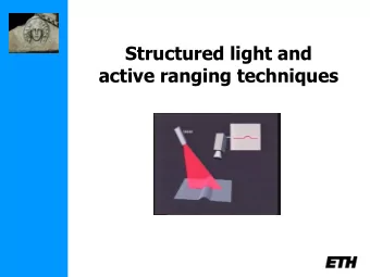
Structured light and active ranging techniques
Today’s class Obtaining “depth maps” / “range images” • unstructured light • structured light • time-of-flight Registering range images (some slides from Szymon Rusinkiewicz, Brian Curless)
Taxonomy 3D modeling passive active photometric … stereo stereo laser structured/ scanning unstructured shape from light silhouettes
Unstructured light project texture to disambiguate stereo
Space-time stereo Davis, Ramamoothi, Rusinkiewicz, CVPR’03
Space-time stereo Davis, Ramamoothi, Rusinkiewicz, CVPR’03
Space-time stereo Zhang, Curless and Seitz, CVPR’03
Space-time stereo Zhang, Curless and Seitz, CVPR’03 • results
Light Transport Constancy Davis, Yang, Wang, ICCV05
Triangulation Light / Laser Camera “Peak” position in image reveals depth
Triangulation: Moving the Camera and Illumination • Moving independently leads to problems with focus, resolution • Most scanners mount camera and light source rigidly, move them as a unit, allows also for (partial) pre-calibration
Triangulation: Moving the Camera and Illumination
Triangulation: Extending to 3D • Alternatives: project dot(s) or stripe(s) Object Laser Camera
Triangulation Scanner Issues • Accuracy proportional to working volume (typical is ~ 1000:1) • Scales down to small working volume (e.g. 5 cm. working volume, 50 µ m. accuracy) • Does not scale up (baseline too large…) • Two-line-of-sight problem (shadowing from either camera or laser) • Triangulation angle: non-uniform resolution if too small, shadowing if too big (useful range: 15 ° -30 ° )
Triangulation Scanner Issues • Material properties (dark, specular) • Subsurface scattering • Laser speckle • Edge curl • Texture embossing Where is the exact (subpixel) spot position ?
Space-time analysis Curless ‘95
Space-time analysis Curless ‘95
Projector as camera
Multi-Stripe Triangulation • To go faster, project multiple stripes • But which stripe is which? • Answer # 1: assume surface continuity e.g. Eyetronics’ ShapeCam
Kinect • Infrared „projector“ • Infrared camera • Works indoors (no IR distraction) • „invisible“ for human Depth Map: Color Image IR Image note stereo shadows! (unused for depth)
Kinect • Projector Pattern „strong texture“ • Correlation-based stereo between IR image and projected pattern possible Homogeneous region, stereo shadow Bad SNR / too close ambiguous without pattern
Multi-Stripe Triangulation • To go faster, project multiple stripes • But which stripe is which? • Answer # 2: colored stripes (or dots)
Multi-Stripe Triangulation • To go faster, project multiple stripes • But which stripe is which? • Answer # 3: time-coded stripes
Time-Coded Light Patterns • Assign each stripe a unique illumination code over time [Posdamer 82] Time Space
Better codes… • Gray code Neighbors only differ one bit = > “Structured light” presented afterwards
Poor man’s scanner Bouguet and Perona, ICCV’98
Pulsed Time of Flight • Basic idea: send out pulse of light (usually laser), time how long it takes to return 1 = 2 ∆ d c t
Pulsed Time of Flight • Advantages: • Large working volume (up to 100 m.) • Disadvantages: • Not-so-great accuracy (at best ~ 5 mm.) • Requires getting timing to ~ 30 picoseconds • Does not scale with working volume • Often used for scanning buildings, rooms, archeological sites, etc.
Depth cameras 2D array of time-of-flight sensors e.g. Canesta’s CMOS 3D sensor jitter too big on single measurement, but averages out on many (10,000 measurements ⇒ 100x improvement)
3D modeling • Aligning range images • Pairwise • Globally (some slides from S. Rusinkiewicz, J. Ponce,…)
Aligning 3D Data • If correct correspondences are known (from feature matches, colors, …), it is possible to find correct relative rotation/translation
Aligning 3D Data ’ X 1 ’ X 2 X 1 X 2 For T as general 4x4 matrix: T Linear solution from ≥5 corrs. e.g. Kinect motion T is Euclidean Transform: X i ’ = T X i 3 corrs. (using quaternions) [Horn87] “Closed-form solution of absolute orientation using unit quaternions”
Aligning 3D Data • How to find corresponding points? • Previous systems based on user input, feature matching, surface signatures, etc.
Spin Images • [Johnson and Hebert ’97] • “Signature” that captures local shape • Similar shapes → similar spin images
Computing Spin Images • Start with a point on a 3D model • Find (averaged) surface normal at that point • Define coordinate system centered at this point, oriented according to surface normal and two (arbitrary) tangents • Express other points (within some distance) in terms of the new coordinates
Computing Spin Images • Compute histogram of locations of other points, in new coordinate system, ignoring rotation around normal: α = p × ˆ “radial dist.” n β = p ⋅ ˆ “elevation” n
Computing Spin Images “elevation” “radial dist.”
Spin Image Parameters • Size of neighborhood • Determines whether local or global shape is captured • Big neighborhood: more discriminative power • Small neighborhood: resilience to clutter • Size of bins in histogram: • Big bins: less sensitive to noise • Small bins: captures more detail
Alignment with Spin Image • Compute spin image for each point / subset of points in both sets • Find similar spin images = > potential correspondences • Compute alignment from correspondences ⇒ Same problems as with image matching: - Robustness of descriptor vs. discriminative power - Mismatches = > robust estimation required
Solving 3D puzzles with VIPs SI FT features VI P features • Extracted from 2D images • Extracted from 3D model • Variation due to viewpoint • Viewpoint invariant (Wu et al., CVPR08) 43
Aligning 3D Data Alternative: assume closest points correspond to each other, compute the best transform…
Aligning 3D Data … and iterate to find alignment Iterated Closest Points (ICP) [Besl & McKay 92] Converges if starting position “close enough“
ICP Variant – Point-to-Plane Error Metric • Using point-to-plane distance instead of point-to- point lets flat regions slide along each other more easily [Chen & Medioni 92]
Finding Corresponding Points • Finding closest point is most expensive stage of ICP • Brute force search – O(n) • Spatial data structure (e.g., k-d tree) – O(log n) • Voxel grid – O(1), but large constant, slow preprocessing
Finding Corresponding Points • For range images, simply project point [Blais/Levine 95] • Constant-time, fast • Does not require precomputing a spatial data structure
Efficient ICP • “Efficient Variants of the ICP algorithm” [Rusinkiewicz & Levoy, 3DIM 2001] = > Presented afterwards
Presentations [Scharstein/Szeliski ‘03]: “High Accuracy Stereo Depth Maps using Structured Light” [Rusinkiewicz/Levoy ‘01]: “Efficient Variants of the ICP Algorithm”
Recommend
More recommend
Explore More Topics
Stay informed with curated content and fresh updates.
