3. Lecture Fourier Transformation Sampling Some slides taken from - PowerPoint PPT Presentation
3. Lecture Fourier Transformation Sampling Some slides taken from Digital Image Processing: An Algorithmic Introduction using Java, Wilhelm Burger and Mark James Burge Separability The 2D DFT can be separated in two 1D DFT's: M 1 N
3. Lecture Fourier Transformation Sampling Some slides taken from “Digital Image Processing: An Algorithmic Introduction using Java”, Wilhelm Burger and Mark James Burge
Separability ² The 2D DFT can be separated in two 1D DFT's: M ¡ 1 N ¡ 1 1 X X f ( x; y ) e ¡ j 2 ¼ ( ux=M + vy=N ) F ( u; v ) = MN x =0 y =0 2 3 M ¡ 1 N ¡ 1 1 4 e ¡ j 2 ¼ux=M 1 X X f ( x; y ) e ¡ j 2 ¼vy=N = 5 M N x =0 y =0 ² The DFT can be obtained in two successive ap- plications of 1D transforms 2
Separability ² First compute the 1D DFT's for all the rows ² Second compute the 1D DFT's for all the columns ² And each of the 1D DFT's can be carried out as FFT of course 3
Separability ² Also the inverse transform can be separated: M ¡ 1 N ¡ 1 X X F ( u; v ) e j 2 ¼ ( ux=M + vy=N ) f ( x; y ) = u =0 v =0 2 3 M ¡ 1 4 e j 2 ¼ux=M N ¡ 1 X X F ( u; v ) e j 2 ¼vy=N = 5 u =0 v =0 4
Example: Separability ² Matlab example using the 2D FFT function: fft2(magic(3)) ans = 45.0000 0 0 0 + 0.0000i 13.5000 + 7.7942i 0.0000 - 5.1962i 0 - 0.0000i 0.0000 + 5.1962i 13.5000 - 7.7942i ² Matlab example using two 1D FFT function calls: fft(fft(magic(3)).').' ans = 45.0000 0 0 0 + 0.0000i 13.5000 + 7.7942i 0.0000 - 5.1962i 0 - 0.0000i 0.0000 + 5.1962i 13.5000 - 7.7942i 5
Symmetry and periodicity ² If f ( x; y ) is real (e.g. an image), its Fourier transform is conjugate symmetric ² Additionally the DFT is in¯nitely periodic 6
Symmetry and periodicity ² The same property holds for the 2D case 7
Translation in the Fourier domain ² A translation ( u 0 ; v 0 ) in the Fourier domain re- sult in ) f ( x; y ) e j 2 ¼ ( u 0 x + v 0 y ) =N F ( u ¡ u 0 ; v ¡ v 0 ) ( ² The origin of the Fourier domain is shifted to the point ( u 0 ; v 0 ) ² A special case is u 0 = v 0 = N= 2, here the ex- ponential term e j¼ ( x + y ) ¡ 1 x + y f ( x; y )( ¡ 1) x + y ( ) F ( u ¡ N= 2 ; v ¡ N= 2) ² The origin will be moved from (0 ; 0) to the cen- tre of the image 8
Example: Translation 9
Rotation ² A rotation in the spatial domain rotates the Fourier domain by the same angle and vice versa. 10
Examples: DFT image scaling. The rectangular pulse in the image function (a – c) creates a strongly oscillating power spectrum (d – f), as in the one- dimensional case. Stretching the image causes the spectrum to contract and vice versa. 11
Examples: DFT — oriented, repetitive patterns. The image function (a – c) contains patterns with three dominant orientations, which appear as pairs of corresponding frequency spots in the spectrum (c – f). Enlarging the image causes the spectrum to contract. 12
Examples: DFT — image rotation. The original image (a) is rotated by 15deg (b) and 30deg (c). The corresponding (squared) spectrum turns in the same direction and by exactly the same amount (d – f). 13
Examples: DFT — superposition of image patterns. Strong, oriented subpatterns (a – c) are easy to identify in the corresponding spectrum (d – f). Notice the broadband effects caused by straight structures, such as the dark beam on the wall in (b, e). 14
Examples: DFT — natural image patterns. Examples of repetitive structures in natural images (a – c) that are also visible in the corresponding spectrum (d – f). 15
Examples: DFT — natural image patterns with no dominant orientation. The repetitive patterns contained in these images (a – c) have no common orientation or sufficiently regular spacing to stand out locally in the orresponding Fourier spectra (d – f). 16
Examples: DFT of a print pattern. The regular diagonally oriented raster pattern (a, b) is clearly visible in the corresponding power spectrum (c). It is possible (at least in principle) to remove such patterns by erasing these peaks in the Fourier spectrum and reconstructing the smoothed image from the modified spectrum using the inverse DFT. 17
Correcting the geometry Correcting the geometry of the 2D spectrum. Original image (a) with dominant oriented patterns that show up as clear peaks in the corresponding spectrum (b). Because the image and the spectrum are not square ( M = N), orientations in the image are not the same as in the actual spectrum (b). After the spectrum is scaled to square size (c), we can clearly observe that the cylinders of this (Harley-Davidson V-Rod) engine are really spaced at a 60 ◦ angle. 18
Windowing Effects of periodicity in the 2D spectrum. The discrete Fourier transform is computed under the implicit assumption that the image signal is periodic along both dimensions (top). Large differences in intensity at opposite image borders — here most notably in the vertical direction — lead to broad-band signal components that in this case appear as a bright line along the spectrum’s vertical axis (bottom). 19
Windowing 20
Fourier basis functions ² Fourier transform represents signal in terms of sine and cosine (basis functions) ² Magnitude gives frequency, direction gives orientation ² Fourier basis element e ¡ j 2 ¼ ( ux + vy ) = cos(2 ¼ ( ux + vy )) ¡ j sin(2 ¼ ( ux + vy )) 21
Fourier basis functions ² Here u and v are larger than in the previous slide 22
Fourier basis functions ² And larger still 23
Fourier basis functions ² Fourier basis elements e ¡ j 2 ¼ ( ux + vy ) = cos(2 ¼ ( ux + vy )) ¡ j sin(2 ¼ ( ux + vy )) 24
Convolution and Correlation ² Convolution: Operator on two sequences that represents a ¯ltering operation ² Correlation: Correlation is a measure of simi- larity between two signals 25
Discrete Convolution ² M ¡ 1 f ( x ) ¤ g ( x ) = 1 X f ( m ) g ( x ¡ m ) M m =0 ² M ¸ A + B ¡ 1 where A is the length of f and B is the length of g ² M ¡ 1 N ¡ 1 1 X X f ( x; y ) ¤ g ( x; y ) = f ( m; n ) g ( x ¡ m; y ¡ n ) MN m =0 n =0 ² A £ B and C £ D are the arrays for f ( x; y ) and g ( x; y ) M ¸ A + C ¡ 1 N ¸ B + D ¡ 1 26
Example: Convolution 27
Example: 2D convolution 28
Discrete Correlation ² The correlation of two functions f ( x ) and g ( x ) is: M ¡ 1 1 D : f ( x ) ± g ( x ) = 1 X f ¤ ( m ) g ( x + m ) M m =0 M ¡ 1 N ¡ 1 1 X X f ¤ ( m; n ) g ( x + m; y + n ) 2 D : f ( x; y ) ± g ( x; y ) = MN m =0 n =0 ² ¤ is the complex conjugate 29
Correlation theorem A correlation in the spatial domain is a multipli- cation with the complex conjugate in the Fourier domain and vice versa. f ( x ) ± g ( x ) , F ¤ ( u ) G ( u ) f ( x; y ) ± g ( x; y ) , F ¤ ( u; v ) G ( u; v ) and f ¤ ( x ) g ( x ) , F ( u ) ± G ( u ) f ¤ ( x; y ) g ( x; y ) , F ( u; v ) ± G ( u; v ) 30
Example: Correlation 31
Example: 2D correlation 32
Sampling ² Sampling can be described as the multiplication of a signal with a sequence of impulse functions 33
Sampling with the impulse function 34
The comb function 35
The comb function 36
Sampling in Fourier domain ² Multiplication of signal with comb function in time domain, is convolution of them in Fourier domain g ( x ) III ( x ) , G ( u ) ¤ III ( u ) 37
Sampling: Fourier domain f(x) A X x 0 38
Reconstruction filters Square pixels Gaussian reconstruction filter 50 50 50 50 100 100 100 100 150 150 150 150 200 200 200 200 250 250 250 50 100 150 200 250 250 50 100 150 200 250 50 100 150 200 250 50 100 150 200 250 Fourier Fourier spatial spatial Bilinear interpolation Perfect reconstruction filter 50 50 50 50 100 100 100 100 150 150 150 150 200 200 200 200 250 250 250 250 50 100 150 200 250 50 100 150 200 250 50 100 150 200 250 50 100 150 200 250 Fourier spatial Fourier spatial 39
Image reconstruction: pixelization square pixels Harmon & Julesz 1973 Gaussian reconstruction 40
Sampling: Aliasing effect 41
Nyquist theorem ² Nyquist theorem: The sampling frequency must be at least twice the highest frequency ! s ¸ 2 ! ² If this is not the case the signal needs to be bandlimited before sampling, e.g. with a low- pass ¯lter 42
Aliasing effect ² Sampling without smoothing: Top row shows the images, sampled at every second pixel to get the next; bottom row shows the magnitude spectrum of these images. ² Nyquist criterium not ful¯lled (aliasing artifacts) 43
Aliasing effect ² Sampling with smoothing: We get the next im- age by smoothing the image with a Gaussian with sigma 1 pixel, then sampling at every sec- ond pixel. 44
Recommend
More recommend
Explore More Topics
Stay informed with curated content and fresh updates.
