? ? 21 22 21 22 Andr es Bruhn Thomas Brox 23 24 23 24 - PowerPoint PPT Presentation

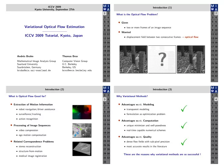
M I M I ICCV 2009 Introduction (1) Kyoto University, September 27th A A 1 2 1 2 What is the Optical Flow Problem? 3 4 3 4 5 6 5 6 � Given 7 8 7 8 Variational Optical Flow Estimation • two or more frames of an image sequence 9 10 9 10 � Wanted 11 12 11 12 ICCV 2009 Tutorial, Kyoto, Japan • displacement field between two consecutive frames → optical flow 13 14 13 14 15 16 15 16 17 18 17 18 19 20 19 20 ? ? 21 22 21 22 Andr´ es Bruhn Thomas Brox 23 24 23 24 Mathematical Image Analysis Group Computer Vision Group 25 26 25 26 Saarland University U.C. Berkeley Saarbr¨ ucken, Germany Berkeley, US 27 28 27 28 1 2 1 2 bruhn@mia.uni-saarland.de brox@eecs.berkeley.edu 29 30 29 30 31 32 31 32 33 33 M I M I Introduction (2) Introduction (3) A A 1 2 1 2 What is Optical Flow Good for? Why Variational Methods? 3 4 3 4 5 6 5 6 � Extraction of Motion Information � Advantages w.r.t. Modeling � 7 8 7 8 • robot navigation/driver assistance • transparent modeling 9 10 9 10 • surveillance/tracking • formulation as optimization problem 11 12 11 12 • action recognition 13 14 13 14 � Advantages w.r.t. Computation � 15 16 15 16 � Processing of Image Sequences • unique minimizer and well-posedness 17 18 17 18 • video compression • real-time capable numerical schemes 19 20 19 20 • ego motion compensation � 21 22 Advantages w.r.t. Quality 21 22 � 23 24 23 24 � • dense flow fields with sub-pixel precision Related Correspondence Problems 25 26 25 26 • stereo reconstruction • most accurate results in the literature 27 28 27 28 • structure-from-motion 29 30 29 30 These are the reasons why variational methods are so successful ! • medical image registration 31 32 31 32 33 33

M I M I ICCV 2009 Tutorial Introduction (4) A Andr´ es Bruhn, Thomas Brox: Variational Optical Flow Computation A 1 2 1 2 Outline of this Tutorial 3 4 3 4 PART I 5 6 5 6 � Part I: Variational Basics ( Andr´ es Bruhn ) Variational Basics 7 8 7 8 • Continuous modeling 9 10 9 10 • Method of Horn and Schunck 11 12 11 12 13 14 13 14 � Part II: Modeling Aspects ( Thomas Brox ) Contents 15 16 15 16 • Motion discontinuities 17 18 17 18 1. Continuous Modeling and Aperture Problem • Robust data terms 19 20 19 20 2. The Method of Horn and Schunck • Large displacements 21 22 21 22 3. Minimization of and Discretization 23 24 23 24 � Part III: Efficient Numerics ( Andr´ es Bruhn ) 4. Solving Linear Systems of Equations 25 26 25 26 • Improved non-hierarchical solvers 27 28 27 28 • Linear and nonlinear multigrid 29 30 29 30 • Implementations on parallel hardware 31 32 31 32 � 2009 Andr´ c es Bruhn, Thomas Brox 33 33 M I M I Continuous Modeling (1) Continuous Modeling (2) A A 1 2 1 2 Continuous Modeling Standard Preprocessing 3 4 3 4 5 6 5 6 � Idea : In order to reduce the influence of noise and outliers, we convolve I 0 with a � Given 7 8 Gaussian K σ of mean µ = 0 and standard deviation σ 7 8 location ( x, y ) ∈ Ω • continuous image sequence I 0 ( x, y, t ) 9 10 9 10 time ∈ [0 , T ] t I ( x, y, t ) = K σ ∗ I 0 ( x, y, t ) 11 12 11 12 � Wanted   13 14 13 14 • image sequence becomes infinitely many times differentiable, i.e. I ∈ C ∞ u ( x, y, t )  → optical flow • interframe displacement field w ( x, y, t ) = v ( x, y, t ) 15 16 15 16  • allows to estimate larger displacements due to the blurring of objects 1 17 18 17 18 19 20 19 20 21 22 21 22 Kσ ∗ 23 24 → 23 24 ◮ 25 26 25 26 27 28 27 28 29 30 29 30 31 32 31 32 I 0 ( x, y, t ) w ( x, y, t ) I 0 ( x, y, t + 1) Important for methods that rely on the computation of image derivatives! 33 33

M I M I Continuous Modeling (3) Continuous Modeling (4) A A 1 2 1 2 The Gray Value Constancy Assumption The Aperture Problem 3 4 3 4 5 6 5 6 � � Idea: In order to retrieve corresponding pixels in subsequent frames, we assume The BCCE provides only one equation for determining two unknowns that their gray value does not change over time: 7 8 7 8 � Ill-posed problem with infinitely many solutions 9 10 9 10 � I ( x + u, y + v, t + 1) − I ( x, y, t ) = 0 . Only the flow component in direction of the image gradient can be computed, 11 12 11 12 the so-called normal flow : n = − I t ∇ I 13 14 13 14 ( u, v ) ⊤ |∇ I | . The Linearized Gray Value Constancy Assumption |∇ f | 15 16 15 16 � This problem is referred to as the aperture problem . It can be illustrated as 17 18 17 18 � Idea: If u and v are small and I is sufficiently smooth, one may linearize this 19 20 19 20 constancy assumption via a first-order Taylor expansion around the point ( x, y, t ) : 21 22 21 22 I ( x + u, y + v, t + 1) ≈ I ( x, y, t ) + I x ( x, y, t ) u + I y ( x, y, t ) v + I t ( x, y, t )1 23 24 23 24 25 26 25 26 → I x u + I y v + I t = 0 . 27 28 27 28 Case I Case II 29 30 29 30 This constraint is the brightness constancy constraint equation (BCCE) . In general such constraints on the flow are called optical flow constraints (OFCs). |∇ I | � = 0 → Aperture problem |∇ I | = 0 → No estimation possible 31 32 31 32 33 33 M I M I Continuous Modeling (5) Continuous Modeling (6) A A 1 2 1 2 Intermezzo I - How to Visualize Optical Flow Fields? Intermezzo II - How to Measure the Quality of Optical Flow Fields? 3 4 3 4 5 6 5 6 Given : estimated flow field w e and ground truth flow field w t � Vector Plot: Subsample vector field and use arrows for visualization � 7 8 7 8 9 10 � Spatiotemporal Average Angular Error (AAE) : 9 10 11 12 11 12 • Consider angle and magnitude by using the spatiotemporal angle 13 14 13 14 � ⊤ w e � N M w t 1 � � 15 16 i,j i,j 15 16 AAE = arccos . | w t | w e i,j | i,j | NM 17 18 17 18 i =1 j =1 19 20 19 20 � Color Plot: Visualize direction as color and magnitude as brightness 21 22 � Average Endpoint Error (AEE) : 21 22 23 24 • Consider the Euclidean distance between the vectors 23 24 25 26 25 26 N M 1 � � | w t i,j − w e 27 28 27 28 AEE = i,j | . NM i =1 j =1 29 30 29 30 31 32 31 32 33 33

M I M I Continuous Modeling (7) Variational Optical Flow Computation (1) A A 1 2 1 2 Variational Optical Flow Computation How Accurate is the Normal Flow? 3 4 3 4 5 6 5 6 What is a Functional? 7 8 7 8 � Known: A function maps an input value to an output value, e.g. 9 10 9 10 11 12 11 12 f ( x, y ) = x 2 + y 2 . 13 14 13 14 15 16 15 16 � New: A functional maps an input function to an output value, e.g. 17 18 17 18 � E ( f ( x, y )) = 1 19 20 19 20 f ( x, y ) dx dy . | Ω | 21 22 21 22 AAE=55.56 ◦ AAE=55.56 ◦ Ω 23 24 23 24 � Remarks: Functionals 25 26 25 26 • can be used to rate the quality of a function w.r.t. certain assumptions 27 28 27 28 • form the basis of variational optical flow methods Results for the Yosemite Sequence with clouds (L. Quam). (a) Upper Left: Frame 8. (b) Upper Right: 29 30 29 30 Frame 9. (c) Lower Left: Ground truth. (d) Lower Right: Normal flow. 31 32 31 32 33 33 M I M I Variational Optical Flow Computation (2) The Method of Horn and Schunck (1) A A 1 2 1 2 Principle of Variational Optical Flow Methods The Method of Horn and Schunck 3 4 3 4 5 6 5 6 � Idea: Compute displacement field as minimizer of a suitable energy functional: � Idea: Assume overall smoothness of the resulting flow field 7 8 7 8 � � The method of Horn and Schunck computes the optical flow as minimizer of 9 10 9 10 E ( u, v ) = D ( u, v ) + S ( u, v ) α dx dy . (Horn/Schunck AI 1981) � �� � � �� � 11 12 11 12 data term smoothness term Ω � + α ( |∇ u | 2 + |∇ v | 2 ) ( I x u + I y v + I t ) 2 E ( w ) = dx dy . 13 14 13 14 � � �� � �� � • data term D ( u, v ) penalizes deviations from constancy assumptions smoothness term data term Ω 15 16 15 16 • smoothness term S ( u, v ) penalizes dev. from smoothness of the solution 17 18 17 18 • data term penalizes deviations from the linearized brightness constancy • regularization parameter α > 0 determines the degree of smoothness 19 20 19 20 assumption (BCCE) 21 22 21 22 • smoothness term penalizes deviations from smoothness of the flow field, 23 24 23 24 � Remarks: The minimising functions u and v i.e. from variations of the functions u and v given by their first derivatives 25 26 25 26 • fit best to all model assumptions (smallest value for the energy functional) 27 28 27 28 • can be seen as a compromise between all (partly contradictive) assumptions Why variational methods can compute a solution everywhere? 29 30 29 30 31 32 31 32 33 33