2 ( ) ( ) Q n n ( , { } 1 ) E IM PM A IM - PowerPoint PPT Presentation
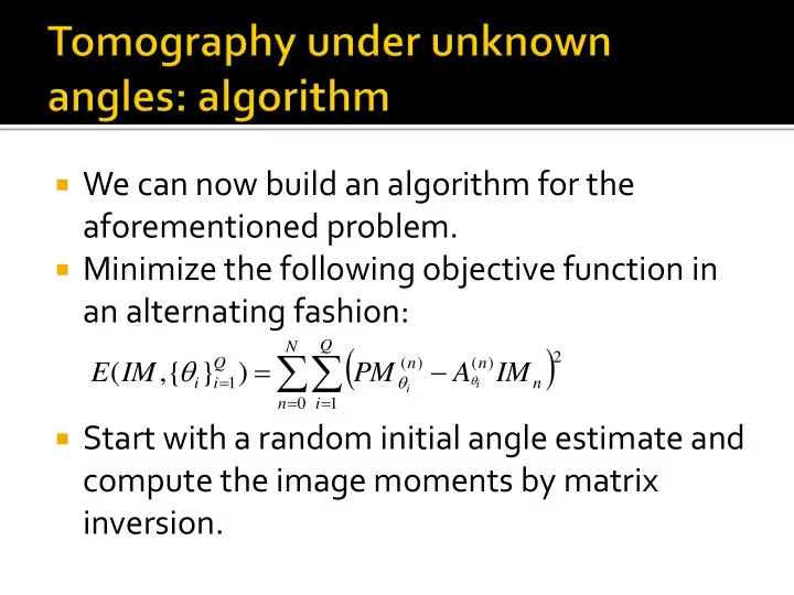
We can now build an algorithm for the aforementioned problem. Minimize the following objective function in an alternating fashion: Q N 2 ( ) ( ) Q n n ( , { } 1 ) E IM PM A IM
We can now build an algorithm for the aforementioned problem. Minimize the following objective function in an alternating fashion: Q N 2 ( ) ( ) Q n n ( , { } 1 ) E IM PM A IM i i n i i 0 1 n i Start with a random initial angle estimate and compute the image moments by matrix inversion.
In other words, systems of equations of the following form have a unique solution in the angles and the image moments, but modulo the rotation ambiguity: n ( ) ( ) n n l l n ( , ) cos sin PM C n l M A IM , i i n l l n i i 0 l Image Column vector of Projection moments moments image moments of order n This is the n -th row of a matrix and it represents the linear combination coefficients for moments of order n and at angle θ i .
Image source: Malhotra and Rajwade, “Tomographic reconstruction with unknown view angles exploiting moment-based relationships” https://www.cse.iitb.ac.i n/~ajitvr/eeshan_icip201 6.pdf
Advantage: simple, makes direct use of the consistency conditions and works even if the number of angles is small Disadvantage: moments are highly sensitive to noise
In this approach, the tomographic projections are “sorted” – i.e. arranged in order of increasing angles. The method relies on the availability of a large number of tomographic projections – all under unknown angles – but sampled independently from a uniform distribution on a unit circle. Given sufficiently many projections, the angles can be assumed to be equi-spaced.
The problem reduces to projection association – i.e. matching each projection to one of the angles, sampled evenly from the unit circle. If the angles are spaced sufficiently closely, and the variation of the projections w.r.t. angle, is smooth, then we can employ a nearest neighbour type of heuristic. This algorithm is summarized on the next slide.
Let us denote the list of available projections as L. Let q i be the i -th tomographic projection and s i be the i -th tomographic projection in the sorted list. WLOG, define the orientation of q 1 to be 0 and set s 1 =q 1 . Find the nearest neighbour of q 1 in L as follows: 2 2 arg min min( , ) r q s q s 1 1 q L reverse or s q q 2 reverse (delete from ) L L q q L Repeat the earlier two steps with s 2 . Continue these steps until L is empty.
At the end of this algorithm, each projection will be associated with an angle at a grid point on the even sampling pattern from 0 to π . Remember: these angles can be estimated only up to a global angular offset which is indeterminate. Following the angle estimates, the underlying image can be reconstructed using FBP.
Note that essentially, each projection is being assigned an angle ranging from 0 to π in steps of π /Q where Q is the number of projections. The aforementioned algorithm is an approximate solution for the well-known travelling salesman problem in computer science. The role of q reverse is to flip projections whose angles would have been in [ π ,2 π ] because g( s , θ + π )=g(- s , θ ) as per the definition of the Radon transform.
The accuracy of the angle estimate increases as the number of angles increases. Consider the k -th order statistic θ (k) , i.e. the k -th largest angle in the sorted sequence. The mean value of this order statistic is 2 π k / Q where Q is the number of angles, assuming uniform distribution of the angles. The variance of this order statistic can be proved to be O(1/ Q 2 ). This method also relies on the fact that the angles were uniformly distributed, otherwise the angle grid points will need to be chosen differently – as per the order statistics of the other distribution.
Usually, the projection angles are unknown, but so are the projection shifts – due to uncontrolled translation of the object being imaged. However the unknown shifts can be solved for using a pre-processing step that assumes that the object is surrounded by vacuum. The tomographic projections can be normalized such that their centroid lies at the origin. The projection ordering step is performed later.
Given tomographic projections of a 2D image in 8 or more distinct and unknown angles, the image moments of order 1 and 2, as well as the angles can be uniquely recovered – but up to the aforementioned rotation ambiguity. This result is true for almost any 2D image (i.e. barring a set of very rare “corner case” images). This result was proved in 2000 by Basu and Bresler at UIUC in a classic paper called “Uniqueness of tomography with unknown view angles”. In an accompanying paper called “Feasibility of tomography with unknown view angles”, they also proved that these estimates are stable under noise. The proof of the theorem and the discussion of the corner cases is outside the scope of our course.
The order n moment of a tomographic projection at angle θ is defined as follows: Substituting the definition of P θ (s) into M θ (n):
In principle, this method is similar to the ordering-based approach. However instead of doing pairwise searches, a dimensionality reduction step is applied. Each tomographic projection q i (under unknown angles) can be regarded as a high-dimensional vector. A dimensionality reduction method is applied to reduce their dimensionality to two (details later), i.e. q i is mapped to y i =( 1i , 2i ).
Consequently the tomographic projection q i will get mapped to the angle: 1 1 i tan i 2 i These angles are then used as estimates of the true angles, prior to FBP-based reconstruction.
We need a method of dimensionality reduction which “preserves the neighbourhood structure” of the original high dimensional points. In order words, if q i and q j were close, their lower- dimensional projections y i and y j should also be close. To define “closeness” mathematically, consider the following proximity matrix W : 2 q q Higher values for W ij means q i i j exp W and q j are nearby in the ij 2 Euclidean sense. Lower values means q i and q j are far apart.
Let the lower-dimensional projections be in 1D for now, i.e. each y i is a scalar. To determine the projections, we now optimize the following: Q 2 Q ({ } ) ( ) E y W y y 1 i i ij i j , i j 2 2 2 y W y W y y W i ij j ij i j ij , , , i j i j i j Define , D W L D W ii ij j 1 Q y t ({ } ) 2 E y Ly i i
So this becomes a constrained minimization problem: t t * arg min such that 1 y y Ly y Dy y The constraint is to prevent the trivial solution. The trivial solution can also be prevented by imposing a unit norm constraint on y , however the one used in the equation above assigns greater importance to points which are “popular”, i.e. for which the D value is high.
So this becomes a constrained minimization problem: t t * arg min such that 1 y y Ly y Dy y The solution to this problem is obtained as follows: ~ t t ( ) ( 1 ) E y y Ly - y D y ~ E 0 Ly D y y This is a generalized eigenvalue problem, and we are interested in the generalized eigenvector y with the smallest generalized eigenvalue (why?).
Now consider that the lower-dimensional points were no longer just in 1D. In such a case, we seek to minimize: Q 2 Q ({ } ) E y W y y i i 1 ij i j , i j t t t 2 y y W y y W y y W i i ij j j ij i j ij , , , i j i j i j T where ( | | ... | ) trace Y L Y Y y y y 1 2 N Normalizat ion constraint : T Y D Y I
This reduces to a generalized eigenvalue problem, i.e. to finding generalized eigenvectors of the following form, with the lowest eigenvalues: Ly Dy This technique is called “Laplacian Eigenmaps ” since the matrix L is called the (graph) Laplacian matrix, which is commonly used in spectral graph theory. This technique is due to Belkin and Niyogi – their NIPS 2003 paper “Laplacian Eigenmaps for Dimensionality Reduction and Data Representation”.
Image source: https://people.cs.pitt.edu/~milos/co urses/cs3750/lectures/class17.pdf
Image source: https://people.cs.pitt.edu/ On this slide, N refers to the number of nearest neighbors per point ~milos/courses/cs3750/lect (the other distances are set to infinity). The parameter for the ures/class17.pdf Gaussian kernel needs to be selected carefully, especially if N is high.
Recommend
More recommend
Explore More Topics
Stay informed with curated content and fresh updates.
