2. Introduction, part two Optimization hierarchy Available solvers - PowerPoint PPT Presentation

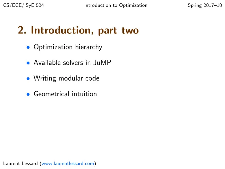
CS/ECE/ISyE 524 Introduction to Optimization Spring 2017–18 2. Introduction, part two ❼ Optimization hierarchy ❼ Available solvers in JuMP ❼ Writing modular code ❼ Geometrical intuition Laurent Lessard (www.laurentlessard.com)

Optimization hierarchy Optimization models can be Models: LP, QP, SOCP, SDP, categorized based on: MIP, IP, MINLP, NLP,... ❼ types of variables ❼ types of constraints Algorithms: gradient descent, ❼ type of objective simplex, interior point method, quasi-Newton methods,... Example: every linear program (LP) has: ❼ continuous variables Solvers: CPLEX, Mosek, Gurobi, ❼ linear constraints ECOS, Clp, Knitro, Ipopt,... ❼ a linear objective Modeling languages: YALMIP, We will learn about many CVX, GAMS, AMPL, JuMP,... other types of models. 2-2

Optimization hierarchy Numerical (usually iterative) Models: LP, QP, SOCP, SDP, procedures that can solve MIP, IP, MINLP, NLP,... instances of optimization models. More specialized Algorithms: gradient descent, algorithms are usually faster. simplex, interior point method, quasi-Newton methods,... generic generality Solvers: CPLEX, Mosek, Gurobi, ECOS, Clp, Knitro, Ipopt,... specialized Modeling languages: YALMIP, slow fast speed CVX, GAMS, AMPL, JuMP,... 2-3

Optimization hierarchy Solvers are implementations Models: LP, QP, SOCP, SDP, of algorithms. Sometimes MIP, IP, MINLP, NLP,... they can be quite clever! ❼ typically implemented in Algorithms: gradient descent, C/C ++ or Fortran simplex, interior point method, ❼ may use sophisticated quasi-Newton methods,... error-checking, complex heuristics etc. Solvers: CPLEX, Mosek, Gurobi, Availability varies: ECOS, Clp, Knitro, Ipopt,... ❼ some are open-source ❼ some are commercial Modeling languages: YALMIP, ❼ some have .edu versions CVX, GAMS, AMPL, JuMP,... 2-4

Optimization hierarchy Modeling languages provide Models: LP, QP, SOCP, SDP, a way to interface with MIP, IP, MINLP, NLP,... many different solvers using a common language. Algorithms: gradient descent, ❼ Can be a self-contained simplex, interior point method, language (GAMS, AMPL) quasi-Newton methods,... ❼ Some are implemented in other languages (JuMP in Julia, CVX in Matlab) Solvers: CPLEX, Mosek, Gurobi, ECOS, Clp, Knitro, Ipopt,... Again, availability varies: ❼ some are open-source Modeling languages: YALMIP, ❼ some are commercial CVX, GAMS, AMPL, JuMP,... ❼ some have .edu versions 2-5

Solvers in JuMP Source: http://www.juliaopt.org/JuMP.jl/0.18/installation.html 2-6

Solvers in JuMP Before solving a model, you must specify a solver. You can do this when you declare the model: using JuMP, Clp, ECOS, SCS m = Model(solver = ClpSolver()) m = Model(solver = ECOSSolver()) m = Model(solver = SCSSolver()) You can also declare a blank model and specify the solver later. m = Model() setsolver(m, ClpSolver()) solve(m) setsolver(m, ECOSSolver()) solve(m) 2-7

Solvers in JuMP Before using a solver, you must include the appropriate package: using JuMP, Clp Every solver must be installed before it can be used: Pkg.add("Clp") Some things to know: ❼ Installing a package may take a couple minutes, but it only has to be done once. ❼ The first time you use a package after you install or update it, Julia will precompile it. This will take an extra 5–30 sec. ❼ Keep all your packages up-to-date using Pkg.update() 2-8

Solvers in JuMP Top Brass.ipynb ❼ Try Clp , ECOS , SCS solvers. Is the answer the same? ❼ Compare solvers using the @time(...) macro ❼ What happens if an unsuitable solver is used? 2-9

Speed vs Generality We will see later in the class that these models are nested: LP ⊆ SOCP ⊆ SDP SCS (an SDP solver) is relatively slow at solving LPs because it solves them by first converting them to an SDP! generic generality SCS ECOS specialized Clp slow fast speed 2-10

Writing modular code It is good practice to separate the data from the model . Top Brass 2.ipynb , Top Brass 3.ipynb ❼ Use dictionaries to make the code more modular ❼ Use expressions to make the code more readable ❼ Use NamedArrays for indexing over sets ❼ Try adding a new type of trophy! 2-11

Comparison: GAMS (1) JuMP and GAMS are * TOP BRASS PROBLEM set I/football, soccer/; structurally very similar free variable profit "total profit"; positive variables x(I) "trophies"; * DATA section parameters profit(I) / "football" 12 , "soccer" 9 / wood(I) / "football" 4 , "soccer" 2 / plaques(I) / "football" 1 , "soccer" 1 /; scalar quant_plaques /1750/ quant_wood /4800/ quant_football /1000/ quant_soccer /1500/; * MODEL section equations obj "max total profit" foot "bound on the number of brass footballs used" socc "bound on the number of brass soccer balls used", plaq "bound on the number of plaques to be used", wdeq "bound on the amount of wood to be used"; 2-12

Comparison: GAMS (2) JuMP and GAMS are * CONSTRAINTS structurally very similar obj.. total_profit =e= sum(I, profit(I)*x(I)); foot.. I("football") =l= quant_football; socc.. I("soccer") =l= quant_soccer; plaq.. sum(I,plaques(I)*x(I)) =l= quant_plaques; wdeq.. sum(I,wood(I)*x(I)) =l= quant_wood; model topbrass /all/; * SOLVE solve topbrass using lp maximizing profit; 2-13

Geometry of Top Brass 2 , 500 max 12 f + 9 s f , s s.t. 4 f + 2 s ≤ 4800 2 , 000 f + s ≤ 1750 soccer balls ( s ) 0 ≤ f ≤ 1000 1 , 500 0 ≤ s ≤ 1500 1 , 000 Each point ( f , s ) is a possible decision. 500 feasible set 0 0 500 1 , 000 1 , 500 footballs ( f ) 2-14

Geometry of Top Brass 1 , 500 max 12 f + 9 s f , s 1 , 250 s.t. 4 f + 2 s ≤ 4800 (650, 1100) f + s ≤ 1750 soccer balls ( s ) 1 , 000 0 ≤ f ≤ 1000 0 ≤ s ≤ 1500 750 p = $ p 1 500 = 2 Which feasible point 0 $ , p 0 9 = 0 has the max profit? 0 , 0 $ 0 6 250 0 , 0 p = 12 f + 9 s 0 0 0 250 500 750 1 , 000 footballs ( f ) 2-15