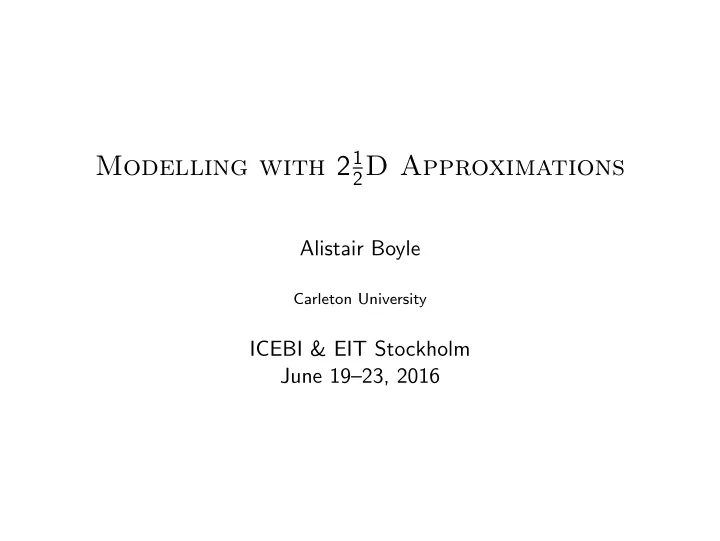
2 D Approximations Alistair Boyle Carleton University ICEBI & - - PowerPoint PPT Presentation

Modelling with 21

2D Approximations

Alistair Boyle

Carleton University

ICEBI & EIT Stockholm June 19–23, 2016

Motivation

2D Models are Wrong

(some of the time)

• A. Boyle, 2016

Carleton University 21/2D Approximations 2 / 13

Motivation

measurement # 5 10 15 20 25 30 35 measurement [Volts] 0.05 0.1 0.15 0.2 0.25 0.3 0.35 0.4 0.45 0.5

analytic FEM 2.5D FEM 3D FEM 2D

2D 21/2-D, 3D, analytic

• A. Boyle, 2016

Carleton University 21/2D Approximations 3 / 13

Motivation

x [m]

• 60
• 40
• 20

20 40 60 80 100 120 140 z [m]

• 150
• 100
• 50

=

2D Models are Still 3D

with a uniform field in z and infinite electrodes

• A. Boyle, 2016

Carleton University 21/2D Approximations 4 / 13

Motivation

=

Electrodes are Finite

but detailed 3d models are expensive

• A. Boyle, 2016

Carleton University 21/2D Approximations 5 / 13

What If

conductivity is uniform in z...

• A. Boyle, 2016

Carleton University 21/2D Approximations 6 / 13

Transform

then we can make use of Fourier transforms

˜ φxy ˜

k =

∞ φxyz cos(˜ kz)dz F (1) −∇ · (σxy∇˜ φxy ˜

k) + ˜

k2σxy˜ φxy˜

k = ˜

Qδxy (2) φxyz = 2 π ∞ ˜ φxy˜

k cos(˜

kz)d˜ k F−1 (3)

• A. Boyle, 2016

Carleton University 21/2D Approximations 7 / 13

Fourier 21

2D

measurement # 5 10 15 20 25 30 35 measurement [Volts] 0.005 0.01 0.015 0.02 0.025 0.03 0.035

analytic FEM 2.5D FEM 3D

21/2-D, analytic 3D

• A. Boyle, 2016

Carleton University 21/2D Approximations 8 / 13

Compute Time

analytic 2D 2 1

2D

3D 1 2 3 4

2 · 10−2 0.23 1.32 3.27

run time [sec]

• A. Boyle, 2016

Carleton University 21/2D Approximations 9 / 13

Compute Time

2D system matrix 0.226 sec fwd solve 0.039 sec 2 1

2D

0.222 sec 0.906 sec for 25 k 3D 2.966 sec 0.149 sec

• A. Boyle, 2016

Carleton University 21/2D Approximations 10 / 13

Another 21

2D Method

with a dual-mesh

x [m]

• 60
• 40
• 20

20 40 60 80 100 120 140 z [m]

• 150
• 100
• 50

+

f

• r

w a r d m

• d

e l inverse model

same geometry but expensive forward solution

• A. Boyle, 2016

Carleton University 21/2D Approximations 11 / 13

Another 2D Method with a dual-mesh

x [m]

• 60
• 40
• 20

20 40 60 80 100 120 140 z [m]

• 150
• 100
• 50

x [m]

• 60
• 40
• 20

20 40 60 80 100 120 140 z [m]

• 150
• 100
• 50

+

forward model inverse model

same geometry but inexpensive forward solution

• A. Boyle, 2016

Carleton University 21/2D Approximations 12 / 13

Fourier 21

2D

Now Available in EIDORS

% fwd_solve: img.fwd_model.solve = @fwd_solve_2p5d_1st_order ;

• img. fwd_solve_2p5d_1st_order .k = [ a .. b ];

% optional

• img. fwd_solve_2p5d_1st_order .method = ’name ’; % optional

% k as integration range , default: [0 Inf] % method as ’trapz ’ ’quadv ’ (default) or ’integral ’ % inv_solve: imdl.fwd_model.solve = @fwd_solve_2p5d_1st_order ; imdl.fwd_model.jacobian = @jacobian_adjoint_2p5d_1st_order ; imdl.fwd_model. system_mat = @system_mat_2p5d_1st_order ;

• A. Boyle, 2016

Carleton University 21/2D Approximations 13 / 13