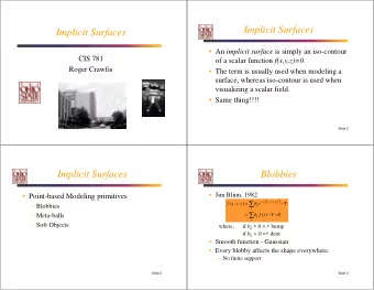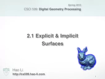
2.1 Explicit & Implicit Surfaces Hao Li - - PowerPoint PPT Presentation

CSCI 621: Digital Geometry Processing

Hao Li

http://cs621.hao-li.com

1

Spring 2019

2.1 Explicit & Implicit Surfaces

Administrative

2

• Exercise 1 discussion: Next Time!
• Hao Li (Instructor)
• Office Hour: Tue 12:30 PM - 1:30 PM, SAL 244
• Zeng Huang (TA)
• Office Hour: TBD, PHE 108
• zenghuan@usc.edu

Last Time

3

Polygonal meshes are

• Effective representations
• Flexible
• Efficient, simple, enables unified processing

Last Time

4

Connection between Meshes and Graphs

• Formalism (valence, connections, subgraph, embedding…)
• Definitions (boundary, regular edge, singular edge, closed mesh)
• triangulation → triangle mesh

A B C D E F G H I J K

Last Time

5

Topology

• Genus, Euler characteristic
• Euler Poincaré formula
• Average valence of triangle mesh: 6
• Triangles: F = 2V, E = 3V
• Quads: F = V, E = 2V

V − E + F = 2(1 − g)

connected k=1 handle ≤2k edge loops

Last Time

6

2-Manifold Surface

• Local Neighborhood is disk-shaped
• Guarantees meaningful neighbor enumeration
• Non-manifold

f(D✏[u, v]) = D[f(u, v)]

Last Time

7

Data Structures

• Face-Based
• Edge-Based, edges always have two faces
• Halfedge-Based

When is a Triangle Mesh a Manifold?

8

• Every Edge incident to 1 or 2 Triangles
• Faces incident to a vertex form closed or open fan

closed fan

• pen fan

Outline

9

• Surface Representations
• Explicit Surfaces
• Implicit Surfaces
• Conversion

Explicit vs. Implicit

10

Explicit:

• Range of parameterization function

f(x) = (r cos(x), r sin(x))T

Implicit:

• Kernel of implicit function

F(x, y) =

• x2 + y2 − r

f([0, 2π]) F(x, y) < 0 F(x, y) > 0 F(x, y) = 0

Explicit vs. Implicit

11

Explicit:

• Range of parameterization function
• Piecewise approximation

F(x, y) =

• x2 + y2 − r

Implicit:

• Kernel of implicit function
• Piecewise approximation

f(x) = (r cos(x), r sin(x))T

? ?

Implicit:

• Kernel of implicit function
• Piecewise approximation
• Scalar-valued 3D grid
• Easy in/out test
• Easy topology modification

Explicit vs. Implicit

12 12

Explicit:

• Range of parameterization function
• Piecewise approximation
• Splines, triangle mesh, points
• Easy enumeration
• Easy geometry modification

Examples: Fluid Simulation

13

Examples: Collisions

14

Examples: 3D Reconstruction

15

Zippering Poisson Reconstruction

Examples: Kinect Fusion

16

http://msdn.microsoft.com/en-us/library/dn188670.aspx

• 1. Capture
• 2. Align
• 3. Fuse

Outline

17

• Surface Representations
• Explicit Surfaces
• Implicit Surfaces
• Conversion

Polynomial Approximation

18

f(t) =

p

• i=0

ci ti =

p

• i=0

˜ ci φi(t) f(ti) = g(ti) , 0 ≤ t0 < · · · < tp ≤ h |f(t) − g(t)| ≤ 1 (p + 1)! max f (p+1)

p

⇤

i=0

(t − ti) = O

• h(p+1)⇥

g(h) =

p

⇤

i=0

1 i! g(i)(0) hi + O

• hp+1⇥

Polynomials are computable functions Taylor expansion up to degree Error for approximation by polynomial

p g f

Spline Surfaces

19

Piecewise polynomial approximation

f (u, v) =

n

• i=0

m

• j=0

cijN n

i (u) N m j (v)

Spline Surfaces

20

Topological constraints

• Rectangular patches
• Regular control mesh

Geometric constraints

• Large number of patches
• Continuity between patches
• Trimming

Piecewise polynomial approximation

Polygon Meshes

21

Polygonal meshes are a good compromise

• Piecewise linear approximation → error is
• Error inversely proportional to #faces
• Arbitrary topology surfaces
• Piecewise smooth surfaces
• Adaptive sampling
• Efficient GPU-based rendering/processing

O(h2)

Triangle Meshes

22

ei, fi ⊂ R3 topology vi ∈ R3

M = ({vi}, {ej}, { fk})

geometry

Outline

23

• Surface Representations
• Explicit Surfaces
• Implicit Surfaces
• Conversion

Implicit Representations

24

Level set of 2D function defines 1D curve

Implicit Representations

25

Level set of 3D function defines 2D surface

Implicit Representations

26

General implicit function:

• Interior:
• Exterior:
• Surface:

Gradient is orthogonal to level set Special case

• Signed distance function (SDF)
• Gradient is unit surface normal

F(x, y) < 0 F(x, y) > 0 F(x, y) = 0

F(x, y, z) < 0 F(x, y, z) > 0 F(x, y, z) = 0 rF rF

Signed Distance Function

27

SDF of a circle? General shapes

SDF Discretization

28

Regular cartesian 3D grid

• Compute signed distance at nodes
• Tri-linear interpolation within cells

F000 (1 − u) (1 − v) (1 − w) + F100 u (1 − v) (1 − w) + F010 (1 − u) v (1 − w) + F001 (1 − u) (1 − v) w + . . . F111 u v w

F000 F100 F010 F110 F111 F011 F101

3-Color Octree

29

1048576 cells 12040 cells 3 Colors: interior,exterior,boundary

Adaptively Sampled Distance Fields

30

12040 cells 895 cells

Binary Space Partitions

31

895 cells 254 cells

Regularity vs. Complexity

32

Implicit surface discretizations

• Uniform, regular voxel grids
• Adaptive, 3-color octrees
• Surface-adaptive refinement
• Feature-adaptive refinement
• Irregular hierarchies
• Binary space partition (BSP)

O(h−3) O(h−2) O(h−1) O(h−1)

Literature

33

• Frisken et al., “Adaptively Sampled Distance Fields: A general

representation of shape for computer graphics”, SIGGRAPH 2000

• Wu & Kobbel, “Piecewise Linear Approximation of Signed Distance

Fields”, VMV 2003

Implicit Representations

34

• Natural representation for volumetric data: CT scans, density

fields, etc.

• Advantageous when modeling shapes with complex and/or

changing topology (e.g., fluids)

• Very suitable representation for Constructive Solid Geometry

(CSG)

CSG Example

35

Union Intersection Difference

FC∪S(·) = min {FC(·) , FS(·)} FC∩S(·) = max {FC(·) , FS(·)} FS\C(·) = max {−FC(·) , FS(·)}

36

CSG Example

CSG Example: Milling

37

Outline

38

• Surface Representations
• Explicit Surfaces
• Implicit Surfaces
• Conversion

Conversion

39

Explicit to Implicit

• Compute signed distance at grid points
• Compute distance point-mesh
• Fast marching

Implicit to Explicit

• Extract zero-level iso-surface
• Other iso-surfaces
• Medical imaging, simulations, measurements, …

F(x, y, z) = 0 F(x, y, z) = C

Signed Distance Computation

40

Find closest mesh triangle

• Use spatial hierarchies (octree, BSP tree)

Distance point-triangle

• Distance to plane, edge, or vertex
• http://www.geometrictools.com

Inside or outside?

• Based on interpolated surface normals

Signed Distance Computation

41

• Closest point
• Interpolated normal
• Inside if

p = αpi + (1 − α)pj n = αni + (1 − α)nj (q − p)>n < 0 q n p pi pj nj

ni

Fast Marching Techniques

42

• Initialize with exact distance in mesh’s vicinity
• Fast-march outwards
• Fast-march inwards

Literature

43

• Schneider, Eberly, “Geometric Tools for Computer Graphics”, Morgan

Kaufmann, 2002

• Sethian, “Level Set and Fast Marching Methods”, Cambridge

University Press, 1999

Conversion

44

Explicit to Implicit

• Compute signed distance at grid points
• Compute distance point-mesh
• Fast marching

Implicit to Explicit

• Extract zero-level iso-surface
• Other iso-surfaces
• Medical imaging, simulations, measurements, …

F(x, y, z) = 0 F(x, y, z) = C

2D: Marching Square

45

• 1. Classify grid nodes as inside/outside
• Is or ?
• 2. Classify cell: 24 configurations
• In/out for each corner
• 3. Compute intersection points
• Linear interpolation along edges
• 4. Connect them by edges
• Look-up table for edge configuration

F(xi,j) > 0 < 0

2D: Marching Square

46

?

3D: Marching Cubes

47

• 1. Classify grid nodes as inside/outside
• Is or
• 2. Classify cell: 28 configurations
• In/out for each corner
• 3. Compute intersection points
• Linear interpolation along edges
• 4. Connect them by edges
• Look-up table for path configuration
• Disambiguation by modified table [Montani ’94]

< 0 F(xi,j,k) > 0

3D: Marching Cubes

48

Classify grid nodes based on

• Inside or outside

Classify all cubes based on

• Inside, outside, or intersecting

Refined only intersected cells

• 3-color adaptive octree
• complexity

O(h−2) Fi,j,k xi,j,k Fi,j,k = F(xi,j,k)

Intersection Points

49

Linear interpolation along edges

xi,j,k · |Fi+1,j,k| + xi+1,j,k · |Fi,j,k| |Fi,j,k| + |Fi+1,j,k|

Intersection Points

50

Linear interpolation along edges

xi,j,k · |Fi,j+1,k| + xi,j+1,k · |Fi,j,k| |Fi,j,k| + |Fi,j+1,k|

Intersection Points

51

Linear interpolation along edges

xi,j,k · |Fi,j,k+1| + xi,j,k+1 · |Fi,j,k| |Fi,j,k| + |Fi,j,k+1|

Intersection Points

52

Linear interpolation along edges Lookup table for patch configuration

Marching Cubes

53

Look-up table with 28 entries

• 15 representative cases shown
• Others follow by symmetry

Marching Cubes

54

Algorithm for isosurface extraction from medical scans (CT, MRI)

Marching Cubes

55

Effect of grid size

Marching Cubes

56

Sample points restricted to edges of regular grid Alias artifacts at sharp features

65×65×65

Increasing Resolution

57

Does not remove alias problems!

Extended Marching Cubes

58

Locally extrapolate distance gradient Place samples on estimated features

65×65×65

Extended Marching Cubes

59

Feature detection

• Based on angle between normals
• Classify into edges / corners

ni

Extended Marching Cubes

60

Feature sampling

• Intersect tangent planes
• Over- or under-determined system
• Solve by SVD pseudo-inverse

    . . . ni . . .     ·   x y z   =     . . . nT

i si

. . .     (si, ni)

Extended Marching Cubes

61

Feature sampling

• Intersect tangent planes
• Triangle fans centered at feature point

(si, ni)

Extended Marching Cubes

62

Feature Detection Feature Sampling Edge Flipping

Milling Simulation

63

257×257×257

CSG Modeling

64

65×65×65

Marching Cubes

65

+ Result is watertight, closed 2-manifold surface! + Easy to parallelize

• Uniform (over-) sampling (→ mesh decimation)
• Degenerate triangles (→ remeshing)
• MC does not preserve features

+ EMC preserves features, but… about 10% more triangles 20-40% computational overhead

Literature

66

• Lorensen & Cline, “Marching Cubes: A High Resolution 3D Surface

Construction Algorithm”, SIGGRAPH 1987

• Montani et al., “A modified look-up table for implicit disambiguation
• f Marching Cubes”, Visual Computer 1994
• Kobbelt et al., “Feature Sensitive Surface Extraction from Volume

Data”, SIGGRAPH 2001

Next Time

67

Discrete Differential Geometry

http://cs621.hao-li.com

Thanks!

68