1st Automotive CFD Prediction Workshop Florian Menter, Chief - PowerPoint PPT Presentation
1st Automotive CFD Prediction Workshop Florian Menter, Chief Scientist Rob Winstanley, Engineering Manager Domenico Caridi, Senior Regional Product Manager Krishna Zore, Software Developer II Tushar Jadhav, Senior Application Engineer GEKO -
1st Automotive CFD Prediction Workshop Florian Menter, Chief Scientist Rob Winstanley, Engineering Manager Domenico Caridi, Senior Regional Product Manager Krishna Zore, Software Developer II Tushar Jadhav, Senior Application Engineer
GEKO - New & Flexible RANS Turbulence Model 2
Motivation • Two-equation models are the work-horse in industrial CFD • The have typically 5 coefficients which can be calibrated to match physics • They are calibrated for ‐ Flat plate boundary layers (log-layer) ‐ Selected free shear flows (plane mixing Central Question: Can we do such a simulation layer, plane jet) with one set of global constants? ‐ Decaying turbulence in freestream Probably not … • Coefficients are linked and cannot be changed easily by user
GEKO Model: Introducing Free Coefficients ( ) ( ) U k k k + = − + + j t P C k The functions F 1 , F 2 , and F 3 contain 6 k t x x x j j k j free coefficients: ( ) ( ) U 2 k + = − + j 2 C F P C F F 1 1 k 2 2 3 t x k x x • C SEP – changes separation behavior j j j • C MIX – changes spreading rates of free + + t x x j j shear flows k • C NW – changes near-wall behavior = ) , ( t max , S C Re al • C JET – Optimizes free jet flows ′ 𝑣 𝑘 ′ 𝑣 𝑗 𝐷 𝐷𝑝𝑠𝑜𝑓𝑠 1.2 𝑢 • C CORNER – Affects corner flows ′ − 𝑇 𝑗𝑙 𝑙𝑘 − 𝑗𝑙 𝑇 𝑙𝑘 ′ 𝑣 𝑘 → 𝑣 𝑗 (𝑇 2 + 2 )/2 𝑁𝐵𝑌 0.3𝜕, • C CURVE – Curvature Correction All coefficients (except C JET ) are UDF functions and can be changed locally
Wall Treatment - Comparison • The formulation of a turbulence model when integrated through the viscous sublayer is a key aspect of turbulence modelling ‐ Defines robustness ‐ Defines accuracy Wall Shear Stress Wall Heat Transfer ‐ Can cause undesired pseudo- Backstep Simulation transition 4x the same k- e model with different near wall treatment • – ML – Menter-Lechner low-Re model – EWT – Enhanced wall treatment built on 2-Layer formulation GEKO-1 exact transformation of k- e to k- with k- wall treatment – V2F - k- e model with V2F ‘elliptic blending’ wall treatment – Makes or Breaks a Turbulence Model • Results are vastly different • GEKO is closest
GEKO Model - Switching • C SEP - active everywhere • C NW - active everywhere (but only relevant near wall) • C MIX – activated by blending function ( ) ... = − • C JET – sub-model of C MIX F C F 1 F MIX MIX JET Blend Wall-Distance Free Variant option available = F 1 Blend
Flat Plate Boundary Layer • Incompressible flow Re = 10 7 ‐ • Variation of C SEP and C NW • Model maintains calibration for wide range of coefficient changes • C MIX and C JET do not affect boundary layer All 4 coefficients can be tuned by user without loss of accuracy for flat plate
Velocity Profiles for CS0 Diffuser: C mix =0 C NW =0.5 Variation of main free coefficients • C NW – affects only near wall – no effect on C p • C SEP – affects separation strength C SEP =1.0 • C MIX – no effect • Main parameter - C SEP
Separated Flow Around a NACA-4412 Airfoil Incompressible flow Flow scheme Re = U ∞ ∙C/ν = 1.64·10 6 C - airfoil chord U ∞ - freestream uniform velocity α = 12 o – angle of attack
Triangular Cylinder – Variation of C MIX – Fixed F GEKO
SEPARATION AND REATTACHMENT AFTER EXPANSION Ahmed Body Incompressible flow Midsection Slant Streamwise velocity contours at the midsection • All the models fail to predict both separation and reattachment on the GEKO-1 GEKO-2 slant • Results of GEKO-1 and GEKO-2 are close to the results of their analog ✓ GEKO- 1 is similar to k−ε SST k- ε Std ✓ GEKO-2 is similar to SST • Results of GEKO-1 and k-e models fit experimental data better than other models
Best Practice Document - GEKO Use 2 nd order turbulence when feasible https://www.ansys.com/- /media/ansys/corporate/resourcelibrary/technical-paper/geko- tp.pdf
Summary - GEKO • A new Generalized k- (GEKO) model has been developed • It allows optimization of free coefficients over a wide range of applications • Instead of switching between different models, users can now adjust a single model to their application • Good chance of consolidation of two-equation models into one optimal format • Further free coefficients will be added • Strong defaults • Coefficients can be changed locally via UDF • Already successfully used in industrial applications • Implementation in Fluent (planned for CFX R20)
Tuning the GEKO Turbulence Model for Case 2a & 2b 25
Tuning the GEKO turbulence model using Design of Experiment • Goal is tuning the GEKO ‐ To improve the prediction of drag and lift on two and eventually on more car models ‐ Using main driving parameters and zonal approach • Car Models used ‐ DrivAer Fastback and DrivAer Estate – Corse Ansa Mesh • Solver Set up ‐ Coupled solver, 2nd order Upwind, LSQ, Pseudo Transient • Parameters used for this study ‐ Csep global ‐ Csep local in the wheel MRF zone ‐ Cmix global 26
Design of Experiment and Optimization using Workbench DX • DOE main set up ‐ Optimal Space Filling Design ‐ 20 samples ‐ Csep range: [1-2] ‐ Cmix range: [0.3-4] • Input parameters ‐ Csep global, Cmix global, Csep local (wheel MRF) • Output parameters ‐ dCD, dCL for Fastback and Estate, dCD Fastback-Estate, Mean Square Error • Total time for one model DOE (20 sim) about 6000 CPU hours ‐ Comparable with one scale resolved simulation • Neural Network Response Surface 27
Results • Multi Objective Genetic Algorithm ‐ Seek for 0 delta for Drag, Lift on both models ‐ Higher priority for Drag ‐ Minimize Mean Square error ‐ Keep same drag trend between two models Very good trade off improvement! 29
Case 2a Coarse – GEKO Csep 1.75 Vs Optimised Csep 1.75 Optimised 0 5 10 15 20 Contours of X Velocity at Plane Y = 0
Case 2a Coarse – GEKO Csep 1.75 Vs Optimised Csep 1.75 Optimised 0 5 10 15 20 Contours of X Velocity at Plane Z = 0
Case 2a Coarse – GEKO Csep 1.75 Vs Optimised Csep 1.75 Optimised -0.9 0 0.9 Contours of Pressure Coefficent
Case 2a Coarse – GEKO Csep 1.75 Vs Optimised 1.00E+00 2.00E+00 5.00E-01 1.50E+00 0.00E+00 1.00E+00 -1.00E+00 -5.00E-01 0.00E+00 5.00E-01 1.00E+00 1.50E+00 2.00E+00 2.50E+00 3.00E+00 3.50E+00 4.00E+00 -5.00E-01 5.00E-01 -1.00E+00 0.00E+00 -1.50E+00 -5.00E-01 -2.00E+00 -1.00E+00 Optimised-pressure-coefficient Csep 1.75-pressure-coefficient z-coordinate
Case 2b Coarse – GEKO Csep 1.75 Vs Optimised Csep 1.75 Optimised 0 5 10 15 20 Contours of X Velocity at Plane Y = 0
Case 2b Coarse – GEKO Csep 1.75 Vs Optimised Csep 1.75 Optimised 0 5 10 15 20 Contours of X Velocity at Plane Z = 0
Case 2b Coarse – GEKO Csep 1.75 Vs Optimised 1.00E+00 2.00E+00 5.00E-01 1.50E+00 0.00E+00 1.00E+00 -1.00E+00 -5.00E-01 0.00E+00 5.00E-01 1.00E+00 1.50E+00 2.00E+00 2.50E+00 3.00E+00 3.50E+00 4.00E+00 -5.00E-01 5.00E-01 -1.00E+00 0.00E+00 -1.50E+00 -5.00E-01 -2.00E+00 -1.00E+00 Optimised-pressure-coefficient Csep 1.75-pressure-coefficient z-coordinate
Mosaic TM Meshing – Case 2a 39
Mosaic (Poly-Hexcore) Meshing Hex Core • High quality • Fast solve time New: Mosaic TM Technology • Unique technology to conformally connect poly prisms to hex • High quality transition, with significantly fewer cells than tet transition • Patent pending Poly Prism • High quality • Significantly fewer cells than tri prisms
Mosaic (Poly-Hexcore) Meshing Parallel – F1 Car • If Fluent Meshing is opened in parallel Distributed Parallel Meshing will auto-enable • Particular benefit for large meshes or number of prism layers • Up to 8.1 Million cells/min with 64-way parallel • Typical memory requirement: <3 GB / Million cells
Mosaic Remeshing of Medium 2a Committee Grid • All wall tri-surfaces unchanged • Quads on MFR Internal Surfaces triangulated and Remeshed • BOI regions and sizing replicated • Prism Layers ‐ Car - 22 Layers, 1.8e-5m first height, variable growth rate to Last Ratio 40% ‐ Road - 22 Layers, first aspect ratio 100, 1.17 growth rate
Mosaic Remeshing of Medium 2a Committee Grid
Recommend
More recommend
Explore More Topics
Stay informed with curated content and fresh updates.
