16623 - Advanced Computer Vision Apps Assignment 3 - Lucas & - PDF document
16623 - Advanced Computer Vision Apps Assignment 3 - Lucas & Kanade Algorithm, Correlation Filters - (15 % of total grade) 100 points - (Q1, Q2, Q3) Released - 19th of October Due - Wednesday 2nd of November (midnight EST) On your local
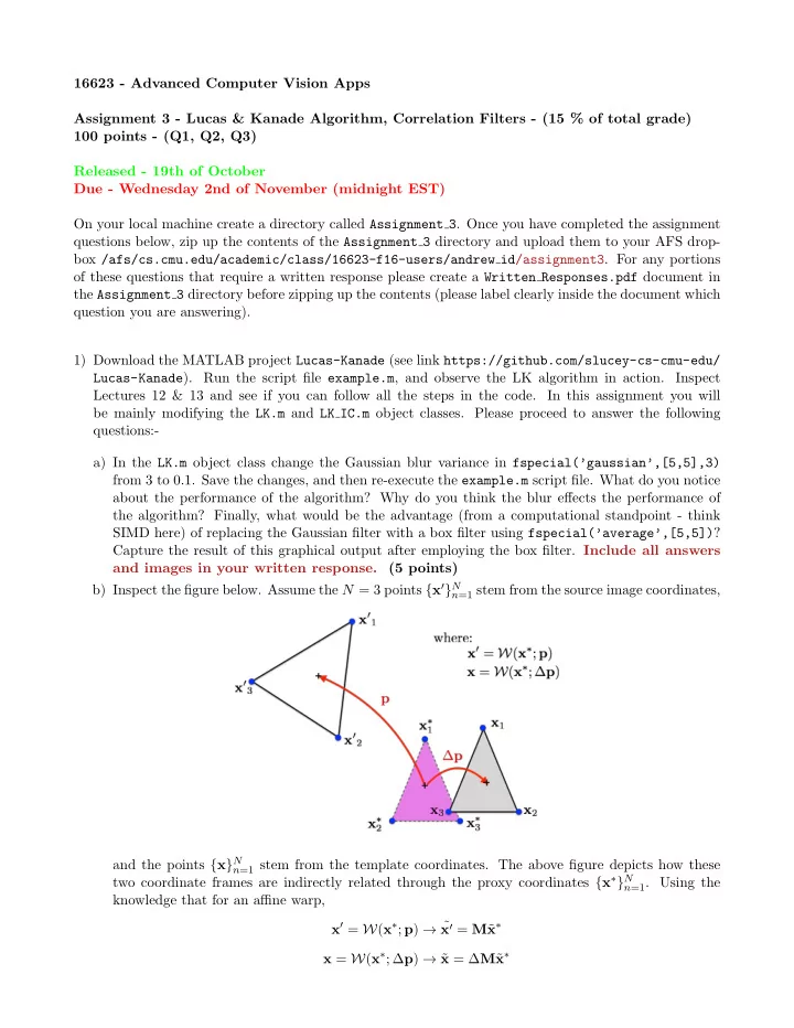
16623 - Advanced Computer Vision Apps Assignment 3 - Lucas & Kanade Algorithm, Correlation Filters - (15 % of total grade) 100 points - (Q1, Q2, Q3) Released - 19th of October Due - Wednesday 2nd of November (midnight EST) On your local machine create a directory called Assignment 3 . Once you have completed the assignment questions below, zip up the contents of the Assignment 3 directory and upload them to your AFS drop- box /afs/cs.cmu.edu/academic/class/16623-f16-users/andrew id/assignment3 . For any portions of these questions that require a written response please create a Written Responses.pdf document in the Assignment 3 directory before zipping up the contents (please label clearly inside the document which question you are answering). 1) Download the MATLAB project Lucas-Kanade (see link https://github.com/slucey-cs-cmu-edu/ Lucas-Kanade ). Run the script file example.m , and observe the LK algorithm in action. Inspect Lectures 12 & 13 and see if you can follow all the steps in the code. In this assignment you will be mainly modifying the LK.m and LK IC.m object classes. Please proceed to answer the following questions:- a) In the LK.m object class change the Gaussian blur variance in fspecial(’gaussian’,[5,5],3) from 3 to 0 . 1. Save the changes, and then re-execute the example.m script file. What do you notice about the performance of the algorithm? Why do you think the blur effects the performance of the algorithm? Finally, what would be the advantage (from a computational standpoint - think SIMD here) of replacing the Gaussian filter with a box filter using fspecial(’average’,[5,5]) ? Capture the result of this graphical output after employing the box filter. Include all answers and images in your written response. (5 points) b) Inspect the figure below. Assume the N = 3 points { x ′ } N n =1 stem from the source image coordinates, and the points { x } N n =1 stem from the template coordinates. The above figure depicts how these two coordinate frames are indirectly related through the proxy coordinates { x ∗ } N n =1 . Using the knowledge that for an affine warp, x ′ = W ( x ∗ ; p ) → ˜ x ′ = M ˜ x ∗ x = W ( x ∗ ; ∆ p ) → ˜ x = ∆ M ˜ x ∗
x = [ x T , 1] T is the representation of x in homogeneous coordinates. where ˜ Demonstrate with x ′ = M ˜ full mathematical working how one would update M using ∆ M such that ˜ x ? Show the mathematical working and all answers in your written response. (5 points) c) The result to the previous question is important as it demonstrates how we can determine the direct relationship between the template image T ( 0 ) and the source image I when we obtain the solution to the indirect relationship, ∆ p ||I ( p ) − T (∆ p ) || 2 arg min 2 which is approximately linearized in practice as, ∆ p ||I ( p ) − T ( 0 ) − T ( 0 ) p T ∆ p || 2 arg min 2 . Based on this result, the Lecture 12-13 notes and reading materials fill in the missing code within the LK IC.m object class file so as to implement an inverse compositional update. Use the class functions p2M and M2p in the provided Affine.m object class to help you with this. If everything is working properly you should be able to swap the LK object for the LK IC object in the example.m script file and re-run everything. Capture the result of this graphical output, this time displaying the bounding box in green. In your own words please describe why the inverse compositional approach is more computationally efficient than the classical forwards additive approach? Include all answers and images in your written response. (20 points) d) In the LK IC.m object class one can note that the imfilter operation is being used with the “replicate” flag being set. Turn the flag off (i.e. just remove it from the function’s input). What does this do to the result? Why is this not an issue with the forwards additive method in the LK.m object class? What could be done to improve the performance of the inverse composition method further in this regard (think of boundary effects and possibly the employment of the conv2 function with the “valid” flag)? Include all answers in your written response. (5 points) 2) Download the MATLAB project Corr-Filters (see link https://github.com/slucey-cs-cmu-edu/ Corr-Filters ). Run the script file example.m , and observe a visual depiction of the extraction of sub-images from the Lena image (Figure 1 in MATLAB) as well as the desired output response from our linear disciminant (Figure 2 in MATLAB). Inspecting example.m you can see that it extracts a set of sub-images X = [ x 1 , . . . , x N ] T from within the Lena image. These sub-images are stored in vector form so that x n ∈ R D (in the example code all the sub-images are 29 × 45 therefore D = 1305). Associated with these images are desired output labels y = [ y 1 , . . . , y N ] where y n lies between zero and one. For this example we have made D = N on purpose. Please proceed to answer the following questions:- a) A linear least-squares discriminant can be estimated by solving N 1 � 2 || y n − x T n g || 2 arg min 2 g n =1 we can simplify this objective in vector form and include an additional penalty term 1 2 + λ 2 || y − X T g || 2 2 || g || 2 arg min (1) 2 . g Please write down the solution to Equation 1 in terms of the matrices S = XX T , X and y . Place the answer in your written response. (5 points)
b) Add your solution to Equation 1 in the example.m code. Visualize the resultant linear discriminant weight vector g using the MATLAB function imagesc for the penalty values λ = 0 and λ = 1 (remember to use the reshape command to convert g back into a 2D array). Apply the filter to the entire Lena image using the imfilter function. Visualize the responses using imagesc for both values of λ . Include these visualizations in your written response document. Can you comment on which value of λ performs best and why? Place your answers and figures in your written response. (5 points) c) Visualize the response you get if you attempt to use the 2D convolution function conv2 with the “same” flage. Why does this get a different response to the one obtained using imfilter ? How could you use the MATLAB operations flipud and fliplr to get a response more similar to the one obtained using imfilter ? Place the answer in your written response. (5 points) 3) Inspect the following properties of circulant Toeplitz matrices and the Fourier transform. Property 1: the D × D Fourier transform matrix F is a scaled orthobasis therefore 2 = 1 || x || 2 x || 2 D || ˆ 2 which is commonly referred to as Pareseval’s theorem. Since ˆ x = F{ x } = Fx is the Fourier D F T ˆ transform therefore x = F − 1 { x } = 1 x is the inverse Fourier transform. Property 2: that a circulant Toeplitz matrix X can be formed from any vector x ∈ R D such that, X ( m, n ) = x (mod { m − n, D } ) . See a description of the mod operator/function in MATLAB. Property 3: that a circulant Toeplitz matrix can always be diagonalized by, X = 1 x ) F = 1 D F T diag(ˆ x } ) F T D F diag(conj { ˆ where x ∈ R D is the vector from which the circulant Toeplitz matrix X was formed. Property 4: that the multiplication of any two circulant Toeplitz matrices X and Y is itself a circu- lant Toeplitz matrix Z , XY = Z . Property 5: properties 1-4 apply not only to circular shifts in one dimension, but to N -dimensional circular shifts. For example a circulant Toeplitz matrix X 2 D formed from 2D circular shifts is diagonalized by a 2D Fourier transform matrix F 2 D (as per property 3). In this assignment all practical examples will involve 2D signals (i.e. images) and therefore 2D circular shifts. The 2 D subscript, however, will be omitted herein. For exampe, if you wanted to apply a 2D FFT matrix transform F to a vectorized 2D image patch a = vec( A ) you would do this in MATLAB through the line, >> Af = fft2(A); where A is the 2D image patch, and ˆ A (which is expressed as Af in MATLAB) is the unvectorized a = vec( ˆ 2D FFT of A such that ˆ A ) = Fa . Now run the script file example circshift.m , and observe a visual depiction of the extraction of circular-shifted sub-images from the Lena image (Figure 1 MATLAB) as well as the desired output response from our linear discriminant (Figure 2 MATLAB). Please proceed to answer the following questions:-
Recommend
More recommend
Explore More Topics
Stay informed with curated content and fresh updates.
