16. Mean Square Estimation Given some information that is related to - PowerPoint PPT Presentation

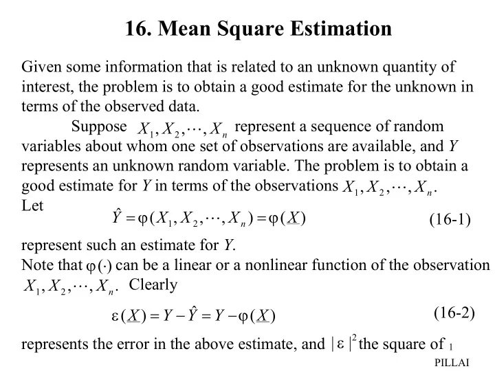
16. Mean Square Estimation Given some information that is related to an unknown quantity of interest, the problem is to obtain a good estimate for the unknown in terms of the observed data. Suppose represent a sequence of random X , X , � , X 1 2 n variables about whom one set of observations are available, and Y represents an unknown random variable. The problem is to obtain a good estimate for Y in terms of the observations X , X , � , X . 1 2 n Let ˆ = ϕ = ϕ Y ( X , X , � , X ) ( X ) (16-1) 1 2 n represent such an estimate for Y . ϕ ( ⋅ Note that can be a linear or a nonlinear function of the observation ) Clearly X , X , � , X . 1 2 n ˆ (16-2) ε = − = − ϕ ( X ) Y Y Y ( X ) | ε 2 | represents the error in the above estimate, and the square of 1 PILLAI

ε 2 ε E { | | } the error. Since is a random variable, represents the mean square error. One strategy to obtain a good estimator would be to minimize the mean square error by varying over all possible forms ϕ ( ⋅ ), of and this procedure gives rise to the Minimization of the Mean Square Error (MMSE) criterion for estimation. Thus under ϕ ( ⋅ ) MMSE criterion,the estimator is chosen such that the mean square error is at its minimum. ε 2 E { | | } Next we show that the conditional mean of Y given X is the best estimator in the above sense. Theorem1: Under MMSE criterion, the best estimator for the unknown Y in terms of is given by the conditional mean of Y X , X , � , X 1 2 n gives X . Thus ˆ = ϕ = Y ( X ) E { Y | X }. (16-3) ˆ Proof : Let represent an estimate of Y in terms of = ϕ Y ( X ) = ˆ Then the error and the mean square X ( X , X , � , X ). ε = Y − Y , 1 2 n error is given by 2 ˆ σ ε = ε = − = − ϕ 2 2 2 2 E { | | } E { | Y Y | } E { | Y ( X ) | } (16-4) PILLAI

Since = (16-5) E [ z ] E [ E { z | X }] X z we can rewrite (16-4) as σ ε = − ϕ = − ϕ 2 2 2 E { | Y ( X ) | } E [ E { | Y ( X ) | X }] � �� �� � �� �� X Y z z where the inner expectation is with respect to Y , and the outer one is with respect to X . Thus σ ε = − ϕ 2 2 E [ E { | Y ( X ) | X }] + ∞ ∫ = − ϕ 2 E { | Y ( X ) | X } f ( X ) dx . (16-6) X − ∞ ϕ , To obtain the best estimator we need to minimize in (16-6) σ 2 ε ϕ ≥ . with respect to In (16-6), since f X ( X ) 0 , − ϕ ≥ 2 E { | Y ( X ) | X } 0 , ϕ and the variable appears only in the integrand term, minimization ϕ σ 2 of the mean square error in (16-6) with respect to is ε 2 X ϕ . − ϕ equivalent to minimization of with respect to E { | Y ( X ) | } 3 PILLAI

ϕ Since X is fixed at some value, is no longer random, ( X ) 2 X and hence minimization of is equivalent to − ϕ E { | Y ( X ) | } ∂ − ϕ = 2 E { | Y ( X ) | X } 0 . (16-7) ∂ ϕ This gives − ϕ = E {| Y ( X ) | X } 0 or − ϕ = E { Y | X } E { ( X ) | X } 0 . (16-8) But ϕ = ϕ E { ( X ) | X } ( X ), (16-9) = ϕ ϕ since when is a fixed number Using (16-9) X x , ( X ) ( x ). 4 PILLAI

in (16-8) we get the desired estimator to be ˆ = ϕ = = Y ( X ) E { Y | X } E { Y | X , X , � , X }. (16-10) 1 2 n Thus the conditional mean of Y given represents the best X , X , � , X 1 2 n estimator for Y that minimizes the mean square error. The minimum value of the mean square error is given by σ = − = − 2 2 2 E { | Y E ( Y | X ) | } E [ E { | Y E ( Y | X ) | X } ] min � � � � � � � � � � � var( Y X ) = ≥ E {var( Y | X )} 0 . (16-11) As an example, suppose is the unknown. Then the best Y = 3 X MMSE estimator is given by ˆ = = = 3 3 Y E { Y | X } E { X | X } X . (16-12) ˆ Y = Y = Clearly if then indeed is the best estimator for Y 3 3 X , X 5 PILLAI

in terms of X . Thus the best estimator can be nonlinear. Next, we will consider a less trivial example. Example : Let < < <  kxy , 0 x y 1 = f ( x , y )  0 otherwise, X , Y  where k > 0 is a suitable normalization constant. To determine the best estimate for Y in terms of X , we need f ( y | x ). Y | X y = ∫ 1 1 ∫ = f ( x ) f ( x , y ) dy kxydy X X , Y x x 1 1 − 2 2 kxy kx ( 1 x ) = = < < , 0 x 1. x 2 2 1 x Thus f ( x , y ) kxy 2 y = = = < < < f ( y | x ) ; 0 x y 1 . X , Y − − 2 2 Y X f ( x ) kx ( 1 x ) / 2 1 x X (16-13) Hence the best MMSE estimator is given by 6 PILLAI

1 ˆ ∫ = ϕ = = Y ( X ) E { Y | X } y f ( y | x ) dy Y | X x 1 1 ∫ ∫ = = 2 y 2 y dy y dy 2 2 2 − − 1 x 1 x x x 1 3 − 3 + + 2 2 y 2 1 x 2 ( 1 x x ) = = = . (16-14) − − − 2 2 2 3 1 x 3 1 x 3 1 x x Once again the best estimator is nonlinear. In general the best estimator is difficult to evaluate, and hence next we E { Y | X } will examine the special subclass of best linear estimators. Best Linear Estimator In this case the estimator is a linear function of the ˆ Y X , X , � , X . observations Thus 1 2 n n ∑ ˆ = + + + = (16-15) Y a X a X � a X a X . l 1 1 2 2 n n i i = i 1 a , a , � , a where are unknown quantities to be determined. The 1 2 n ˆ ε = Y − mean square error is given by ( Y ) 7 l PILLAI

∑ ˆ ε = − = − 2 2 2 E { | | } E {| Y Y | } E { | Y a X | } (16-16) l i i a , a , � , a and under the MMSE criterion should be chosen so 1 2 n ε 2 that the mean square error is at its minimum possible E { | | } σ value. Let represent that minimum possible value. Then 2 n n ∑ σ = − (16-17) 2 2 min E {| Y a X | }. n i i a , a , � , a = 1 2 n i 1 To minimize (16-16), we can equate ∂ ε = = 2 E {| | } 0 , k 1 , 2 , � ,n. (16-18) ∂ a k This gives   *     ∂ ∂ ε ∂ ε 2 | | ε = = ε = 2   E {| | } E 2 E 0 .     (16-19) ∂ ∂ ∂ a a a         k k k But 8 PILLAI

n n ∑ ∑ ∂ − ∂ ( Y a X ) ( a X ) ∂ ε ∂ i i Y i i = = − = − = = i 1 i 1 X . (16-20) k ∂ ∂ ∂ ∂ a a a a k k k k Substituting (16-19) in to (16-18), we get ∂ ε 2 E {| | } = − ε = * 2 E { X } 0 , k ∂ a k or the best linear estimator must satisfy ε = = (16-21) * E { X } 0 , k 1 , 2 , � , n . k ε Notice that in (16-21), represents the estimation error ∑ = n − ( Y a i X ), and represents the data. Thus from = 1 → X k , k n i i 1 ε = 1 → X k , k n (16-21), the error is orthogonal to the data for the best linear estimator. This is the orthogonality principle . In other words, in the linear estimator (16-15), the unknown a , a , � , a constants must be selected such that the error 1 2 n 9 PILLAI

∑ = n ε = − is orthogonal to every data for the Y a i X X , X , � , X i 1 2 n i 1 best linear estimator that minimizes the mean square error. Interestingly a general form of the orthogonality principle holds good in the case of nonlinear estimators also. Nonlinear Orthogonality Rule: Let represent any functional h ( X ) E { Y | X } form of the data and the best estimator for Y given With X . = − e Y E { Y | X } we shall show that = (16-22) E { eh ( X )} 0 , implying that = − ⊥ e Y E { Y | X } h ( X ). This follows since = − E { eh ( X )} E {( Y E [ Y | X ]) h ( X )} = − E { Yh ( X )} E { E [ Y | X ] h ( X ) } = − E { Yh ( X )} E { E [ Yh ( X ) | X ]} = − = E { Yh ( X )} E { Yh ( X )} 0 . 10 PILLAI