1 Outline Chi-square test Logistic regression 2 Chi-square test - PowerPoint PPT Presentation

Dongmei Li Department of Public Health Sciences Office of Public Health Studies University of Hawai’i at Mānoa 1

Outline  Chi-square test  Logistic regression 2

Chi-square test 3

Chi-Square Test - Example Data below reveal a negative association between smoking and education level. Let us test H 0 : no association in the population vs. H a : association in the population. 4

χ 2 , Expected Frequencies  row total column tot al  xpected frequencie s E E i table total 5

Chi-Square Test of Association A. Hypotheses. H 0 : no association in population versus H a : association in population B. Test statistic.   2  O E  2   i i  where observed count, cell O i stat i E i all cells  row total column tot al   and expected count in cell calculated E i E i i table total    ( 1 )( 1 ) df R C C. P -value. Convert the X 2 stat to a P -value with a a Table E or software program. 6

Chi-Square Statistic - Example 7

Chi-Square Test, P -value  X 2 stat = 13.20 with 4 df  Using Chi-square Table, find the row for 4 df  Find the chi-square values in this row that bracket 13.20  Bracketing values are 11.14 (P = .025) and 13.28 (P = .01).  Thus, .025 < P < .01 (closer to .01) Probability in right tail df 0.98 0.25 0.20 0.15 0.10 0.05 0.025 0.01 0.01 4 0.48 5.39 5.99 6.74 7.78 9.49 11.14 13.28 14.86 8

Illustrative example X 2 stat = 13.20 with 4 df The P -value = AUC in the tail beyond X 2 stat 9

Yates’ Continuity Corrected Chi -Square Statistic  Two different chi-square statistics are used in practice  Pearson’s chi -square statistic (covered) is   2  O E  2   i i stat E i all cells  Yates’ continuity -corrected chi-square statistic is:   2   1 | | O E  2 i i   2 stat, c E i all cells  The continuity-corrected method produces smaller chi- square statistics and larger P -values.  Both chi-square are used in practice. 10

Chi-Square test using JMP  Data set: Presentation4_chisqtest.jmp 11

Results from JMP  P-value from both likelihood ratio test and Pearson chi-square test is 0.0103  Significant association between education level and smoking status 12

Chi-Square, cont. How the chi-square works. When observed values 1. = expected values, the chi-square statistic is 0. When the observed minus expected values gets large and evidence against H 0 mounts Avoid chi-square tests in small samples. Do not 2. use a chi-square test when more than 20% of the cells have expected values that are less than 5. Supplement chi-squares with measures of 3. association. Chi-square statistics do not measure the strength of association. Use descriptive statistics or Relative Risks to quantify “strength”. 13

Logistic Regression 14

Logistic regression example  Surviving third-degree burns  These Presentation4_Burn.jmp data refer to 435 adults who were treated for third-degree burns by the University of Southern California General Hospital Burn Center. The patients were grouped according to the area of third-degree burns on the body. (The groups are identified as midpoints of set intervals of log(area +1).) For each patient, it was recorded whether or not they survived, and the area of their burn was recorded as the midpoint of the group corresponding to their burn.  Source: http://statmaster.sdu.dk/courses/st111/module14/index.html 15

Logistic regression example  Variable Description  Midpoint: Midpoint of the group corresponding to the patients burn.  survive: Binary variable: survived=1, died=0  A first idea might be to model the relationship between the probability of success (that the patient survives) and the explanatory variable ‘log(area +1)’ as a simple linear regression model. 16

Logistic regression example  However, the scatterplot of the proportions of patients surviving a third-degree burn against the explanatory variable shows a distinct curved relationship between the two variables, rather than a linear one. It seems that a transformation of the data is in place. 17

Logistic regression example  The curved relationship is typical for many situations where the response variable is binary.  Some examples of the curved relationship 18

Logistic regression example  The following scatterplot shows the logit-transformed proportions of patients surviving a third-degree burn against the explanatory variable ‘log(area +1)’. 19

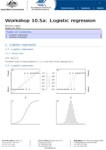
The simple logistic regression model  The simple logistic regression model relates p x to x through the following equation: 1    ( | ) p P D X x   x  ( ) a bx 1 e  Alternatively, it can be written as p     x log( ) log( | ) odds for D X x a bx  1 p x 20

Fit logistic regression in JMP  Data set: Presentation4_Burn.jmp 21

Fit logistic regression in JMP  Estimated logistic regression     log ( ) 22 . 71 10 . 66 int it p midpo 22

Interpretation of logistic regression parameters  If X has several discrete levels or is measured on a continuous scale, there is no change in the interpretation of a (log odds of D when X=0)  The log odds ratio comparing two exposure groups is        | 1 /( 1 ) odds for D X x p p     1 1 x x log( ) log log OR       | /( 1 )  odds for D X x   p p  x x     log[ /( 1 )] log[ /( 1 )] p p p p   1 1 x x x x         [ ( 1 )] [ ] a b x a b x b  b is the log odds ratio associated with a unit increase in X  10.66 is the log odds ratio of death associated with a unit increase in midpoint midpoints of set intervals of log(area +1). 23

Example of logistic regression model  Consider a study of the analgesic effects of treatments on elderly patients with neuralgia. Two test treatments and a placebo are compared. The response variable is whether the patient reported pain or not. Researchers recorded age and gender of the patients and the duration of complaint before the treatment began. The data, consisting of 60 patients, are contained in the data set Presentation4_logistic.jmp.  Look at the difference between male and female on pain  Look at the treatment effect on pain 24

Logistic regression in JMP  Data set: Presentation4_logistic.jmp  Analyze---Fit Model 25

Logistic regression in JMP  Logistic regression results    log ( ) 0 . 37 0 . 63 * ( ) it p I sex F 26

Interpretation of logistic regression parameters  Suppose the exposure variable X only takes on two values (1 is exposed and 0 is unexposed)  When X=0, then log( p 0 /1- p 0 )= a + b *0 = a  So, a is the log odds of D amongst the unexposed.       | 1 /( 1 ) odds for D X p p   1 1 log( ) log log   OR     | 0 /( 1 )  odds for D X   p p  0 0     log[ /( 1 )] log[ /( 1 )] p p p p 1 1 0 0        ( 1 ) ( 0 ) a b a b b  The slope parameter b is just the log Odds Ratio.  0.63 is the log odds ratio of No Pain comparing females vs. males. 27

Odds ratio from JMP  Odds ratio for sex  The odds ratio of reporting no pain comparing females vs. males is 3.60 and the odds ratio could be as low as 1.25 and as high as 11.09 with 95% confidence from the observed data. 28

Odds ratio from JMP  Calculate the odds ratio of no pain for comparing treatment A or B vs. placebo. 29

Exercise  A study is conducted to examine the effect of age on coronary heart disease (CHD). The data includes the ID and the age of the subject and whether the subject has CHD or not.  1. Fit a logistic regression to examine the effect of age on CHD.  2. Fit a logistic regression to examine the effect of age group on CHD.  Data set Presentation4_logisticCHD.jmp. 30

31