13.1 Review of Last Lecture Review of primal and dual of SVM. - PDF document

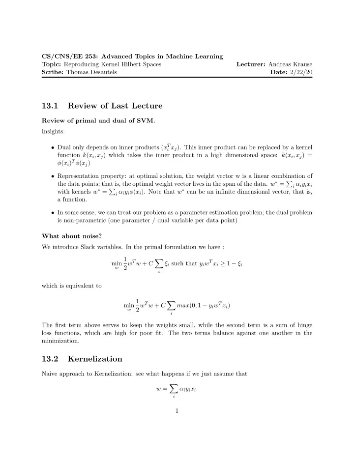
CS/CNS/EE 253: Advanced Topics in Machine Learning Topic: Reproducing Kernel Hilbert Spaces Lecturer: Andreas Krause Scribe: Thomas Desautels Date: 2/22/20 13.1 Review of Last Lecture Review of primal and dual of SVM. Insights: • Dual only depends on inner products ( x T i x j ). This inner product can be replaced by a kernel function k ( x i , x j ) which takes the inner product in a high dimensional space: k ( x i , x j ) = φ ( x i ) T φ ( x j ) • Representation property: at optimal solution, the weight vector w is a linear combination of the data points; that is, the optimal weight vector lives in the span of the data. w ∗ = � i α i y i x i with kernels w ∗ = � i α i y i φ ( x i ). Note that w ∗ can be an infinite dimensional vector, that is, a function. • In some sense, we can treat our problem as a parameter estimation problem; the dual problem is non-parametric (one parameter / dual variable per data point) What about noise? We introduce Slack variables. In the primal formulation we have : 1 2 w T w + C ξ i such that y i w T x i ≥ 1 − ξ i � min w i which is equivalent to 1 2 w T w + C max (0 , 1 − y i w T x i ) � min w i The first term above serves to keep the weights small, while the second term is a sum of hinge loss functions, which are high for poor fit. The two terms balance against one another in the minimization. 13.2 Kernelization Naive approach to Kernelization: see what happens if we just assume that � w = α i y i x i . i 1

Then the optimization problem becomes equivalent to 1 � � � α i α j y i y j x T α j y j x T min α i x j + C max(0 , 1 − y i j x i ) . 2 i,j i j To kernelize, replace x T i x j terms with k ( x i , x j ) When is this appropriate? The key assumption is that w ∈ Span { x i , ∀ i } (which we derived last lecture in the case of no-noise). Let ˜ α i = α i y i Note that we’re unconstrained here: we can flip signs arbitrarily. Then the problem is equivalent to 1 � � � min α i ˜ ˜ α j k ( x i , x j ) + C max (0 , 1 − y i α j k ( x i , x j )) . ˜ 2 α ˜ i,j i j Recall:   k ( x 1 , x 1 ) k ( x 1 , x n ) . . . . . ... . . K =   . .   k ( x n , x 1 ) k ( x n , x n ) . . . This matrix is called the ”Gram Matrix”, and so the above is equivavlent to 1 α T K ˜ � min 2 ˜ α + C max (0 , 1 − y i f ( x i )) α ˜ i where the first term is the complexity penalty and the second term represents the penalty for poor fit, where we use the notation f ( x ) = f α ( x ) = � j ˜ α j k ( x j , x ). Suppose we want to learn a non-linear classifier for the unit interval: one way to do this is to learn a non-linear function f which takes values roughly the labels, st. y i ≈ sign ( f ( x i )) This function could fit this condition only at the datapoints and so look sort of like a comb (with the teeth at the datapoints, and the function otherwise near zero) or it could be a much more smoothly varying function which takes a value in between the datapoints which is similar to close by datapoints. These functions are sketched in Figure 13.2. The complicated, comb-like, high-order function would work, but we would prefer the simpler, smoother function: To ensure goodness-of-fit, we want to have correct prediction with a good margin: | f ( x i ) | > 1. To control complexity, we prefer simpler functions. How can we mathematically express this preference? In general, we want to solve: 1 f ∗ = min 2 || f || 2 + C � l ( f ( x i ) , y i ) f ∈ F i where l is an arbitrary loss function, for example, the hinge loss used above. Questions: what is F? What is the right norm/complexity of the function? 2

+1 -1 Figure 13.2.1: Candidate non-linear classification functions In the following, we will answer these questions. For the definition of || f || that we will derive, it i αk ( x i , · ), it will hold that || f || 2 = α T Kα , i.e., the same penalty will, for functions f = f α = � term as introduced above. In the following, we will assume that l is an arbitrary loss function, i.e., we require that l ( f ( x i ) , y i ) ≥ 0 and if f ( x i ) = y i then l ( f ( x i ) , y i ) = 0. 13.3 Reproducing Kernel Hilbert Spaces Definition 13.3.1 (Hilbert space) Let X be a set (“index set”) A Hilbert space H = H ( X ) is a linear space of functions H : { f : X → R } along with an inner product < f, g > (which implies a norm || f || = √ < f, f > ) which is complete: all Cauchy sequences in H converge to a limit in H . Definition 13.3.2 (Cauchy Sequence) f 1 , . . . , f n is a Cauchy sequence if ∀ ǫ, ∃ n o such that ∀ n, n ′ ≥ n o || f n − f n ′ || < ǫ . The Cauchy sequence f 1 , . . . , f n converges to f if || f n − f || → 0 as n → ∞ . Definition 13.3.3 (RKHS) A Hilbert space is called a Reproducing Kernel Hilbert Space (RKHS) for kernel function k if both of the following conditions are true: (1) any function f ∈ H can be written as an infinite linear combination of kernel evaluations: f = � ∞ i =1 a i k ( x i , · ) for x 1 , . . . , x n ∈ X Note that for any fixed x i , k ( x i , · ) maps X → R (2) H k satisfies the reproducing property: < f, k ( x i , · ) > = f ( x i ) that is, the kernel function clamped to one x i is the evaluating functional for that point. The above definition implies that < k ( x i , · ) , k ( x j , · ) > = k ( x i , x j ) ← − entries in the Gram matrix 3

Example: X = R n H = { f : f ( x ) = w T x for some w ∈ R n } For functions f ( x ) = w T x , g ( x ) = v T x , define < f, g > = w T v Define kernel function (over X ): k ( x, x ′ ) = x T x ′ Verify (1) and (2) (1) Consider f ( x ) = w T x = � n i =1 w i x i = � n i =1 w i k ( e i , x ) where e i is the indicator vector: the unit vector in the i th direction. So (1) is verified. (2) Let f ( x ) = w T x < f, k ( x i , · ) > = w T x i = f ( x i ) so (2) is verified. Note that the first equality holds because k ( x i , x ) = x T i x and k ( x i , x ) is a function on X → R because k : X × X → R . 13.4 Important points on RKHS Questions: (a) Does every kernel k have an associated RKHS? (b) Does every RKHS have a unique kernel? (c) Why is this useful? Answers (a) Yes: k = { f = � n let H ′ i =1 k ( x i , · ) and i,j α i β j k ( x i , x j ) for f = � n i =1 α i k ( x i , · ), g = � m < f, g > = � j =1 β j k ( x j , · ) Check if this satisfies the reproducing property: < f, k ( x ′ , · ) > = � n i =1 α i k ( x, x ′ ) Space H ′ k is not yet complete: add all limits of all cauchy sequences to it to complete it. Then this is an RKHS. Define φ : x → k ( x, · ) consider < φ ( x ) , φ ( x ′ ) > = < k ( x, · ) , k ( x ′ , · ) > = k ( x, x ′ ) Can think of k as an inner product in that RKHS. The above is an explicit way of constructing the high dimensional space for which the kernel function is the inner product. (b) Consider k and k ′ , two positive definite kernel functions which produce the same RKHS. Does k = k ′ ? Yes → next homework assignment. (c) Why is this useful? Return to our original problem: 1 f ∗ = min f ∈ F 2 || f || 2 + � l ( f ( x i ) , y i ) i Let F be an RKHS: F = H k Theorem 13.4.1 For arbitrary (not even convex) loss functions of form above, any optimal so- lution to the problem can be written as a linear combination of these kernel evaluations: for all datasets x i , y i ∃ α 1 , . . . , α n such that f ∗ = � n i =1 α i k ( x i , · ) 4

Proof: Next lecture. The above is from [Kimmeldorf and Wahba]. Representer Theorem: For convex loss functions under strong convexity conditions, the solution is unique. If not strongly convex, but convex, the set of solutions is a convex set. 5