1 Mean Shift Algorithm Graph-Theoretic Image Segmentation Mean - PDF document
6.891 Last time: Segmentation and Clustering (Ch. 14) Computer Vision and Applications Supervised->Unsupervised Category Learning needs segmentation Prof. Trevor. Darrell K-Means Mean Shift Graph cuts Lecture 15:
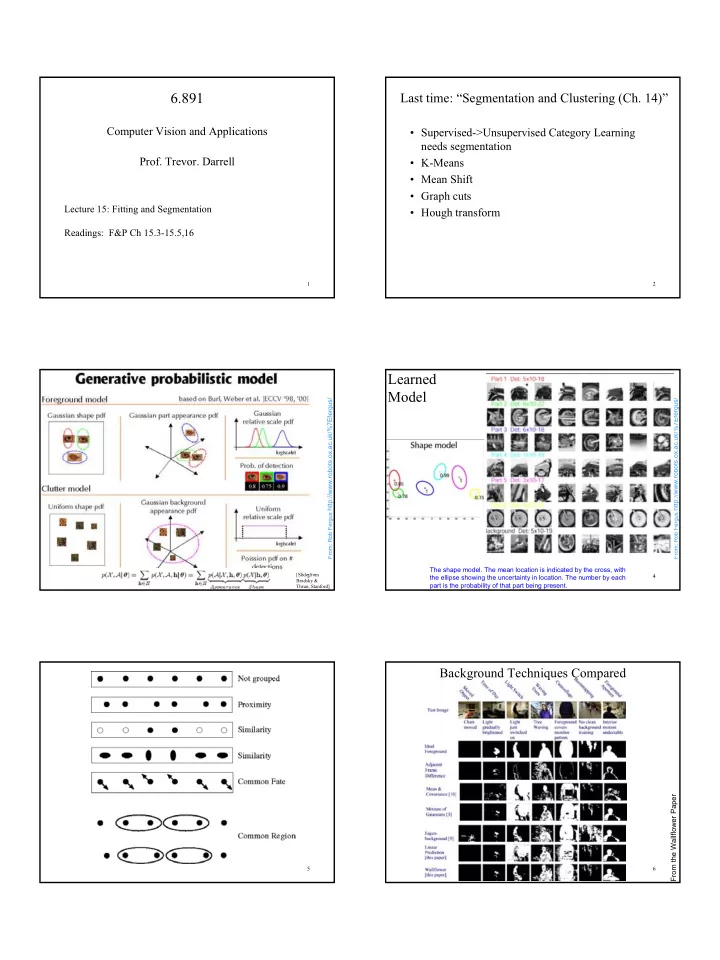
6.891 Last time: “Segmentation and Clustering (Ch. 14)” Computer Vision and Applications • Supervised->Unsupervised Category Learning needs segmentation Prof. Trevor. Darrell • K-Means • Mean Shift • Graph cuts Lecture 15: Fitting and Segmentation • Hough transform Readings: F&P Ch 15.3-15.5,16 1 2 Learned Model From: Rob Fergus http://www.robots.ox.ac.uk/%7Efergus/ From: Rob Fergus http://www.robots.ox.ac.uk/%7Efergus/ The shape model. The mean location is indicated by the cross, with [Slide from 3 4 the ellipse showing the uncertainty in location. The number by each Bradsky & part is the probability of that part being present. Thrun, Stanford] Background Techniques Compared From the Wallflower Paper 5 6 1
Mean Shift Algorithm Graph-Theoretic Image Segmentation Mean Shift Algorithm 1. Choose a search window size. 2. Choose the initial location of the search window. Build a weighted graph G=(V,E) from image 3. Compute the mean location (centroid of the data) in the search window. 4. Center the search window at the mean location computed in Step 3. 5. Repeat Steps 3 and 4 until convergence. V:image pixels The mean shift algorithm seeks the “mode” or point of highest density of a data distribution: E: connections between pairs of nearby pixels W : probabilit y that i & j ij belong to the same region 7 8 Eigenvectors and affinity clusters Hough transform • Simplest idea: we want a • This is an eigenvalue problem - vector a giving the association choose the eigenvector of A between each element and a with largest eigenvalue cluster • We want elements within this cluster to, on the whole, have strong affinity with one another • We could maximize • But need the constraint a T Aa a T a = 1 tokens votes • Shi/Malik, Scott/Longuet- Higgens, Ng/Jordan/Weiss, etc. 9 10 Today “Fitting and Robustness Segmentation (Ch. 15)” • Robust estimation • Squared error can be a source of bias in the presence of noise points • EM – One fix is EM - we’ll do this shortly • Model Selection – Another is an M-estimator • RANSAC • Square nearby, threshold far away – A third is RANSAC (Maybe “Segmentation I” and “Segmentation II” • Search for good points would be a better way to split these two lectures!) 11 12 2
13 14 15 16 Robust Statistics Estimating the mean • Recover the best fit to the majority of the data. Gaussian distribution • Detect and reject outliers. 0 2 3 4 6 Mean is the optimal solution to: 1 N ∑ N µ = d ∑ − µ min ( d ) 2 i N i = i 1 µ i = 1 residual 17 18 3
Estimating the Mean Estimating the mean The mean maximizes this likelihood: 1 N 1 ∏ µ = − − µ 2 σ 2 max p ( d | ) exp( ( d ) / ) i i 2 π σ 2 µ i = 1 The negative log gives (with sigma=1): 0 2 4 6 N ∑ − µ 2 min ( d ) i µ i = 1 “least squares” estimate 19 20 Estimating the mean Influence Breakdown point What happens if we change just one measurement? * percentage of outliers required to make the solution arbitrarily bad. Least squares: 6+ ∆ 0 2 4 ∆ * influence of an outlier is linear ( ∆ /N) µ ' = µ + N * breakdown point is 0% -- not robust! With a single “bad” data point I can move the mean What about the median? arbitrarily far. 0 2 4 6+ ∆ 21 22 What’s Wrong? Approach Influence is proportional to the derivative of the ρ function. N ∑ − µ 2 min ( d ) i µ = i 1 Outliers (large residuals) have too much influence. Want to give less influence to points beyond some value. ρ x = ( ) x 2 ψ = ( x ) 2 x 23 24 4
Approach Approach N N ∑ ∑ ρ − µ σ ρ − µ σ min ( d , ) min ( d , ) i i µ µ i = 1 i = 1 Scale parameter Scale parameter Robust error function Robust error function 2 Replace x ρ σ = σ No closed form solutions! ( x , ) - Iteratively Reweighted Least Squares with something that gives less influence to outliers. - Gradient Descent 25 26 L1 Norm Redescending Function ψ x = ρ x = ( ) sign ( x ) ( ) | x | Tukey’s biweight. Beyond a point, the influence begins to decrease. Beyond where the second derivative is zero – outlier points 27 28 Robust Estimation Robust Estimation Geman-McClure function works well. Twice differentiable, redescending. Influence function (d/dr of norm): 2 σ 2 r 2 r ρ σ = σ ψ σ = σ ( r , ) ( r , ) + 2 + 2 ( 2 r 2 ) 2 r 29 30 5
Robust scale Too small Scale is critical! Popular choice: 31 32 Just right Too large 33 34 Example: Motion Estimating Flow Estimating Flow Assumption: Within a finite image region, there is only a Minimize: single motion present. = ∑ ρ + + σ Violated by: motion discontinuities, shadows, transparency, E ( a ) ( I u ( x ; a ) I v ( x ; a ) I , ) x u t specular reflections… ∈ x R Parameterized models provide strong constraints: * Hundred, or thousands, of constraints. * Handful (e.g. six) unknowns. Can be very accurate (when the model is good)! Violations of brightness constancy result in large residuals: 35 36 6
Deterministic Annealing Continuation method Start with a “quadratic” optimization problem and gradually reduce outliers. GNC: Graduated Non- Convexity 37 38 Fragmented Occlusion Results 39 40 Results Multiple Motions, again X Find the dominant motion while rejecting outliers. Black & Anandan; Black & Jepson 41 42 7
Robust estimation models only a single Alternative View process explicitly * There are two things going on simultaneously. Robust norm: * We don’t know which constraint lines correspond to which ∑ = ρ ∇ + σ motion. T E ( a ) ( I u ( x ; a ) I ; ) t * If we knew this we could estimate the multiple motions. ∈ x , y R - a type of “segmentation” problem Assumption: * If we knew the segmentation then estimating the motion would be easy. Constraints that don’t fit the dominant motion are treated as “outliers” (noise). Problem? They aren’t noise! 43 44 EM General framework Missing variable problems Estimate parameters from segmented data. A missing data problem is a statistical problem where some data is missing There are two natural contexts in which missing Consider segmentation labels to be missing data. data are important: • terms in a data vector are missing for some instances and present for other (perhaps someone responding to a survey was embarrassed by a question) • an inference problem can be made very much simpler by rewriting it using some variables whose values are unknown. 45 46 Missing variable problems Missing variable problems A missing data problem is a statistical problem In many vision problems, if some variables were known the maximum likelihood inference problem where some data is missing would be easy There are two natural contexts in which missing – fitting; if we knew which line each token came from, it data are important: would be easy to determine line parameters • terms in a data vector are missing for some – segmentation; if we knew the segment each pixel came instances and present for other (perhaps from, it would be easy to determine the segment someone responding to a survey was parameters embarrassed by a question) – fundamental matrix estimation; if we knew which • an inference problem can be made very much feature corresponded to which, it would be easy to determine the fundamental matrix simpler by rewriting it using some variables – etc. whose values are unknown. 47 48 8
Strategy Motion Segmentation For each of our examples, if we knew the “What goes with what?” missing data we could estimate the parameters effectively. If we knew the parameters, the missing data would follow. This suggests an iterative algorithm: 1. obtain some estimate of the missing data, using a guess at the parameters; 2. now form a maximum likelihood estimate of the The constraints at these pixels all “go together.” free parameters using the estimate of the missing 49 50 data. Smoothness in layers Layered Representation segmentation [Adelson] 51 52 EM in Pictures EM in Pictures w ( x , y ) I(x,y,t) I(x,y,t) 1 Given images at times t and t+1 Assume we know the containing two motions. segmentation of pixels into “layers” w ( x , y ) I(x,y,t+1) I(x,y,t+1) 2 ≤ ≤ 0 w ( x , y ) 1 i ∑ = w ( x , y ) 1 i i 53 54 9
EM in Pictures EM in Equations I(x,y,t) w ( x , y ) I(x,y,t) w ( x , y ) u ( x , y ; a ) u ( x , y ; a ) 1 1 1 1 1 1 w ( x , y ) I(x,y,t+1) I(x,y,t+1) u ( x , y ; a ) 2 2 2 ∑ = ∇ T + 2 E ( a ) w ( x )( I u ( x ; a ) I ) 1 1 1 t x , y ∈ R Then estimating the motion of each “layer” is easy. 55 56 EM in Equations EM in Pictures I(x,y,t) ∑ = ∇ + E ( a ) w ( x )( I T u ( x ; a ) I ) 2 2 2 2 t x , y ∈ R w ( x , y ) I(x,y,t+1) u ( x , y ; a ) 2 2 2 Ok. So where do we get the weights? 57 58 EM in Pictures EM in Pictures Assume we know the motion of the layers but not the ownership probabilities of the pixels (weights). The weights represent the probability that the constraint “belongs” to a particular layer. 59 60 10
Recommend
More recommend
Explore More Topics
Stay informed with curated content and fresh updates.
