1 Pure Reinforcement Learning vs. Reinforcement Learning - PDF document
CSE 573: Artificial Intelligence Todo Reinforcement Learning Add simulations from 473 Dan Weld Add UCB bound (cut bolzman & constant epsilon Add snazzy videos (pendulum, zico kolter See http://www See http://www-
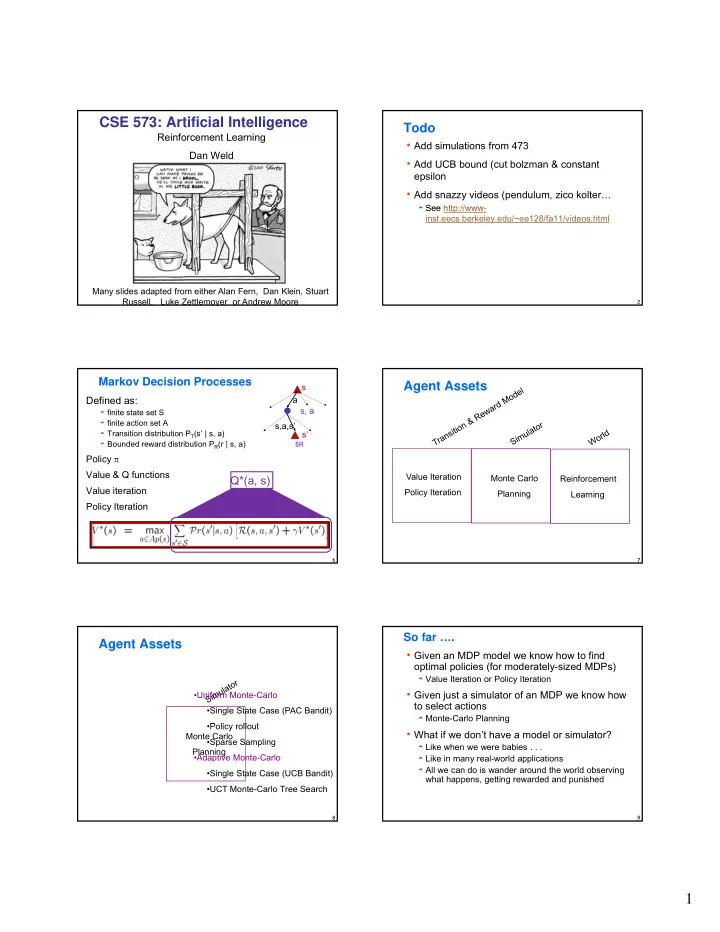
CSE 573: Artificial Intelligence Todo Reinforcement Learning Add simulations from 473 Dan Weld Add UCB bound (cut bolzman & constant epsilon Add snazzy videos (pendulum, zico kolter… See http://www See http://www- inst.eecs.berkeley.edu/~ee128/fa11/videos.html Many slides adapted from either Alan Fern, Dan Klein, Stuart Russell, Luke Zettlemoyer or Andrew Moore 1 2 Markov Decision Processes Agent Assets s Defined as: a s, a finite state set S finite action set A s,a,s’ Transition distribution P T (s’ | s, a) s’ Bounded reward distribution P R (r | s, a) $R Policy Value & Q functions Value Iteration Q*(a, s) Monte Carlo Reinforcement Value iteration Policy Iteration Planning Learning Policy Iteration 6 7 So far …. Agent Assets Given an MDP model we know how to find optimal policies (for moderately-sized MDPs) Value Iteration or Policy Iteration Given just a simulator of an MDP we know how •Uniform Monte-Carlo to select actions •Single State Case (PAC Bandit) Monte-Carlo Planning •Policy rollout P li ll t What if we don’t have a model or simulator? Monte Carlo •Sparse Sampling Like when we were babies . . . Planning •Adaptive Monte-Carlo Like in many real-world applications All we can do is wander around the world observing •Single State Case (UCB Bandit) what happens, getting rewarded and punished •UCT Monte-Carlo Tree Search 8 9 1
Pure Reinforcement Learning vs. Reinforcement Learning Monte-Carlo Planning No knowledge of environment Can only act in the world and observe states and reward In pure reinforcement learning: the agent begins with no knowledge Many factors make RL difficult: wanders around the world observing outcomes Actions have non-deterministic effects In Monte-Carlo planning Which are initially unknown the agent begins with no declarative knowledge of the world Rewards / punishments are infrequent has an interface to a world simulator that allows observing the has an interface to a world simulator that allows observing the Often at the end of long sequences of actions outcome of taking any action in any state How do we determine what action(s) were really responsible for reward or punishment? (credit assignment) The simulator gives the agent the ability to “teleport” to any state, at any time, and then apply any action World is large and complex A pure RL agent does not have the ability to teleport But learner must decide what actions to take Can only observe the outcomes that it happens to reach We will assume the world behaves as an MDP 10 11 Pure Reinforcement Learning vs. Applications Monte-Carlo Planning MC planning aka RL with a “strong simulator” I.e. a simulator which can set the current state Pure RL aka RL with a “weak simulator” Robotic control helicopter maneuvering, autonomous vehicles I.e. a simulator w/o teleport Mars rover - path planning, oversubscription planning elevator planning A strong simulator can emulate a weak simulator Game playing - backgammon, tetris, checkers So pure RL can be used in the MC planning framework Neuroscience But not vice versa Computational Finance, Sequential Auctions Assisting elderly in simple tasks Spoken dialog management Communication Networks – switching, routing, flow control War planning, evacuation planning 12 Model-Based vs. Model-Free RL Passive vs. Active learning Model-based approach to RL: Passive learning learn the MDP model, or an approximation of it The agent has a fixed policy and tries to learn the utilities of use it for policy evaluation or to find the optimal policy states by observing the world go by Analogous to policy evaluation Often serves as a component of active learning algorithms Model-free approach to RL: Model free approach to RL: Often inspires active learning algorithms derive optimal policy w/o explicitly learning the model Active learning useful when model is difficult to represent and/or learn The agent attempts to find an optimal (or at least good) policy by acting in the world Analogous to solving the underlying MDP, but without first We will consider both types of approaches being given the MDP model 14 15 2
Small vs. Huge MDPs Key Concepts Exploration / Exploitation First cover RL methods for small MDPs Number of states and actions is reasonably small Eg can represent policy as explicit table GLIE These algorithms will inspire more advanced methods Later we will cover algorithms for huge MDPs Function Approximation Methods Policy Gradient Methods Least-Squares Policy Iteration 16 17 RL Dimensions RL Dimensions Active Active Many States ADP TD Learning Direct Passive Passive Estimation Uses Model Uses Model Model Free Model Free 18 19 Example: Passive RL RL Dimensions Suppose given a stationary policy (shown by arrows) TD Learning Actions can stochastically lead to unintended grid cell Want to determine how good it is Optimistic Q Learning Explore / RMax ADP -greedy Active ADP TD Learning Direct Passive Estimation Uses Model Model Free 20 21 3
Passive RL Objective: Value Function Estimate V (s) Not given transition matrix, nor reward function! Follow the policy for Follow the policy for many epochs giving training sequences. (1,1) (1,2) (1,3) (1,2) (1,3) (2,3) (3,3) (3,4) +1 (1,1) (1,2) (1,3) (2,3) (3,3) (3,2) (3,3) (3,4) +1 (1,1) (2,1) (3,1) (3,2) (4,2) -1 Assume that after entering +1 or -1 state the agent enters zero reward terminal state So we don’t bother showing those transitions 22 23 Direct Estimation Approach 1: Direct Estimation Converge very slowly to correct utilities values Direct estimation (also called Monte Carlo) (requires a lot of sequences) Estimate V (s) as average total reward of epochs containing s (calculating from s to end of epoch) Reward to go of a state s Doesn’t exploit Bellman constraints on policy values the sum of the (discounted) rewards from that state until a terminal state is reached ( ) ( ) ( , , ' ) ( ' ) V s R s T s a s V s Key: use observed reward to go of the state s ' It is happy to consider value function estimates that violate as the direct evidence of the actual expected this property badly. utility of that state Averaging the reward-to-go samples will How can we incorporate the Bellman constraints? converge to true value at state 24 25 Approach 2: Adaptive Dynamic Programming (ADP) ADP learning curves ADP is a model based approach (4,3) Follow the policy for awhile Estimate transition model based on observations Learn reward function Use estimated model to compute utility of policy (3,3) ( ( ) ) ( ( ) ) ( ( , , ' ) ) ( ( ' ) ) V V s s R R s s T T s s a a s s V V s s ( , ) (2,3) s ' (1,1) (3,1) learned (4,1) (4,2) How can we estimate transition model T(s,a,s’)? Simply the fraction of times we see s’ after taking a in state s. NOTE: Can bound error with Chernoff bounds if we want 26 27 4
Recommend
More recommend
Explore More Topics
Stay informed with curated content and fresh updates.
