1 A comprehensive example Sow replacement in practice At every - PDF document
Outline Short survey of animal replacement models A 4-level model for optimal feeding level, fattening policy and slaughtering of organic steers (BKN): Model structure Decisions being optimized Animal replacement models A 3-level
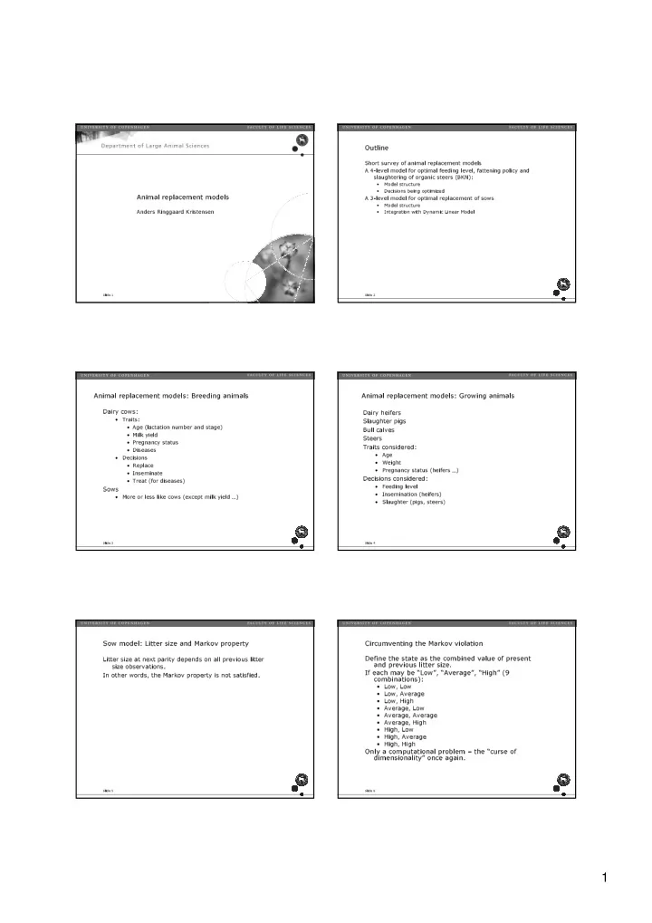
Outline Short survey of animal replacement models A 4-level model for optimal feeding level, fattening policy and slaughtering of organic steers (BKN): • Model structure • Decisions being optimized Animal replacement models A 3-level model for optimal replacement of sows • Model structure • Integration with Dynamic Linear Model Anders Ringgaard Kristensen Slide 1 Slide 2 Animal replacement models: Breeding animals Animal replacement models: Growing animals Dairy cows: Dairy heifers • Traits: Slaughter pigs • Age (lactation number and stage) Bull calves • Milk yield Steers • Pregnancy status Traits considered: • Diseases • Age • Decisions • Weight • Replace • Pregnancy status (heifers …) • Inseminate Decisions considered: • Treat (for diseases) • Feeding level Sows • Insemination (heifers) • More or less like cows (except milk yield …) • Slaughter (pigs, steers) Slide 3 Slide 4 Sow model: Litter size and Markov property Circumventing the Markov violation Define the state as the combined value of present Litter size at next parity depends on all previous litter and previous litter size. size observations. If each may be “Low”, “Average”, “High” (9 In other words, the Markov property is not satisfied. combinations): • Low, Low • Low, Average • Low, High • Average, Low • Average, Average • Average, High • High, Low • High, Average • High, High Only a computational problem – the “curse of dimensionality” once again. Slide 5 Slide 6 1
A comprehensive example Sow replacement in practice At every weaning or return to oestrus it is decided whether or A sow replacement model not to cull the sow. • Developed for practical use at prototype level The decision is based on a prediction of the future • 3 levels: Decisions at 2 levels performance of the sow. • Estimation at herd level The prediction is compared to the expected performance of a gilt. • Bayesian updating (Dynamic linear model) Only based on existing registrations. • Decision making Slide 7 Slide 8 Prediction of sow performance What do we know about litter size in sows? Based on The profile for a herd: • Individual conditions • It is lower for a gilt than for a second parity sow • Age • A maximum is reached at parity 3, 4, 5 • Litter size results (all) • It is decreasing for older sows • Re-matings • Some herds produce at a higher level than others • Herd specific conditions Within herd: • Litter size profile of the herd • Some sows produce at a higher level than others • Level of involuntary replacement • The repeatability over parities is rather low • Piglet mortality • Large random variation • Prices • Feed intake • Standard conditions • Weight of sows Slide 9 Slide 10 A litter size model Litter size profile for a specific herd Toft & Jørgensen (2002) suggested the following litter size model Intercept = θ 3 15 meeting the demands mentioned on the previous slide: Y it = µ t + M i ( t ) + ε it , where θ 1 Slope = θ 4 13 • Y it is the litter size of sow i at parity t µ t = - θ 1 exp(-( t 2 -1) θ 2 ) + θ 3 - θ 4 t is the litter size profile of the Litter size • 11 herd. Curve: θ 2 M i ( t ) ∼ N(0, σ 2 ) is the effect of sow i at parity t • ε it ∼ N(0, τ 2 ) is random variation (noise) • 9 The sow effect is auto correlated over parities: • Cov( M i ( t ), M i ( t+u )) = exp(- u α ) σ 2 , in other words 7 • M i ( t ) = ρ M i ( t -1) + η it , where 1 2 3 4 5 6 7 8 9 10 11 12 ρ = exp(- α ) Parity • η it ∼ N(0, (1- a 2 ) σ 2 ) • Described by 7 herd specific parameters: θ 1 , θ 2 , θ 3 , θ 4 , τ , σ , α Slide 11 Slide 12 2
Between-herd-variation, 8 Danish herds Litter size profile for a specific herd Estimated from herd data 15 Herd level productivity Censoring: 13 • Only the best sows are kept • Profile will be biased if simple Litter size averages are used 11 • A maximum likelihood estimation technique is used 9 7 1 2 3 4 5 6 7 8 9 10 11 12 Parity Slide 13 Slide 14 Between-herd-variation, 7 selected Spanish herds Between-herd-variation, “all” Spanish herds Litter size profiles of selected Spanish sow herds Litter size profiles of Spanish sow herds 13 13 12 12 Average litter size (total) Average litter size (total) 11 11 10 10 9 9 8 8 7 7 1 3 5 7 9 11 1 3 5 7 9 11 Parity Parity Slide 15 Slide 16 The Markov property in sows The Markov property Let i n be the state at stage n Does ”Age” satisfy the Markov property • Yes! The Markov property is satisfied if and only if Does ”Rematings” satisfy the Markov property? • P( i n+ 1 | i n , i n- 1 , … , i 1 ) = P ( i n+ 1 | i n ) • Yes, almost. The probability of conception hardly depends on • In words: The distribution of the state at next stage depends previous results at all. only on the present state – previous states are not relevant. Does ”Litter size” satisfy the Markov property? This property is crucial in Markov decision processes. • No, certainly not. Several high (or low) will further increase (or decrease) our expectations to future litter size. Example: • Sow 1: 12 – 14 – 16 – 15 – 16 piglets • Sow 2: 6 – 5 – 7 – 6 – 16 piglets • We prefer sow 1 Slide 17 Slide 18 3
Litter size profile for a specific herd Litter size prediction for an individual sow Individual sows are compared to 15 Based on: that • Litter size profile of the herd • Sow 1 is below average 13 • Sow 2 is above average • Individual deviations from the litter size profile Litter size The difference between the • All previous litter sizes must be taken into account, 11 observations and the profile is because we don’t know M i ( t ) due to Uncertainty about the prediction is taken into account 9 • The sow effect M i ( t ) The random error ε it • • Not just “average” 7 1 2 3 4 5 6 7 8 9 10 11 12 Parity Sow 1 Sow 2 Slide 19 Slide 20 Lacking Markov property: From registration to information The lacking Markov property must be considered when the state is defined Straight forward solution: • Define the state as i n = ( y 1 , y 2 , … , y n ) • For a sow in parity 8 this means e.g. 15 8 = 2.5 x 10 9 state combinations. • Prohibitive Slide 21 Slide 22 From registrations to information Coping with the Markov property Estimate the litter size parameters θ 1 , θ 2 , θ 3 , θ 4 , Interpretation • Registration: Litter size λ i = y i τ , σ , α of the herd in question. • Data: Λ = { y 1 , y 2 , … , y n } • Processing: Ψ () - Kalman filtering, DLM These parameters are then considered as • Information: I = Ψ ( Λ ) = ( i 1 , i 2 ) known, implying that also the litter size profile µ t = - θ 1 exp(-( t 2 -1) θ 2 ) + θ 3 - θ 4 t is • Decision: Θ • Decision strategy: I → Θ known. Ψ (): As little loss of information as possible Define the deviation for a sow as I t = Y t - µ t = M ( t ) + ε t (preferably none). • Define a Dynamic Linear Model: Observation equation I t = M ( t ) + ε t , ε it ∼ N(0, τ 2 ) • System equation: M i ( t ) = ρ M i ( t -1) + η it , η it ∼ N(0, (1- a 2 ) σ 2 ) • Slide 23 Slide 24 4
The Kalman filter (West & Harrison, 1997) Prediction Applying the Kalman filter to a DLM allows us to estimate M ( t ) ~ N(0, σ 2 ) parity by parity as litter size observations are done. The current estimate m t for M ( t ) is sufficient for prediction. Having observed t parities of a sow, we have that the conditional All information from previous litter size observations is distribution of M ( t ) given all previous observations is included in that. We have E( Y t +1 | Y 1 , … , Y t ) = µ t +1 + ρ m t • At each parity, the distribution is updated according to • Var( Y t +1 | Y 1 , … , Y t ) = V t +1 The variance only depends on the number of observations – not the values observed. It is not necessary to remember all observed litter sizes. The current estimate m t for M ( t ) is sufficient! Thus, we satisfy the Markov property by only one state variable. Slide 25 Slide 26 Biological parameters Model structure Founder level Litter size parameters: • Stage: Life span of a sow • Herd level estimation • State: Dummy • Censoring • Decision: Dummy Other assumptions Child level 1 • Conception rates (parity, remating) • Stage: Production cycle from weaning • Piglet mortality (parity) • State: M ( n ) • Sow weight (parity) • Decision: Mating method • Involuntary culling (parity) • Feed intake Slide 27 Slide 28 Model structure Prototype Child level 2 A plug-in for the MLHMP software • Stages: ”Mating”, ”Gestation”, ”Suckling” Herd interface • State: • Herd specific parameters and prices • Mating: ”Healthy”, ”Diseased” • Reads sow data • Gestation: ”Pregnant”, ”Infertile”, ”Diseased” • Presents results • Suckling: Present litter size Built for use in practice • Decision: Demonstration • Mating: Allow m matings, m ∈ {1,…,5} • Gestation: Dummy • Suckling: ”Keep”, ”Replace” Slide 29 Slide 30 5
DLM and MDP First processing: Monitoring & filtering Second processing: Decision making MDP with DLM integrates both parts Slide 31 6
Recommend
More recommend
Explore More Topics
Stay informed with curated content and fresh updates.

