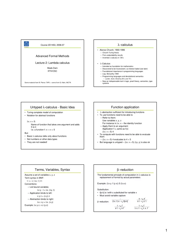

λ− calculus Course 2D1453, 2006-07 • Alonzo Church, 1903-1995 – Church-Turing thesis – First undecidability results Advanced Formal Methods – Invented λ -calculus in ’30’s Lecture 2: Lambda calculus λ -Calculus • – Intended as foundation for mathematics Mads Dam – Discovered to be inconsistent, so interest faded (see later) KTH/CSC – Foundational importance in programming languages – Lisp, McCarthy 1959 – Programming languages and denotational semantics • Landin, Scott, Strachey 60’s and 70’s – Now an indispensable tool in logic, proof theory, semantics, type Some material from B. Pierce: TAPL + some from G. Klein, NICTA systems Untyped λ -calculus - Basic Idea Function application λ -abstraction sufficient for introducing functions • Turing complete model of computation • • To use functions need to be able to • Notation for abstract functions – Refer to them: Use variables x, y, z λ x. x + 5: For instance in λ x. x – the identity function Name of function that takes one argument and adds – Apply them to an argument: 5 to it Application f x, same as f(x) I.e. a function f: x � x + 5 ( λ x. x + 5) 4 But: • To compute with functions need to be able to evaluate • Basic λ -calculus talks only about functions them – ( λ x. x + 5) 4 evaluates to 4 + 5 • Not numbers or other data types • But language is untyped – ( λ x. x + 5) ( λ y. y) is also ok • They are not needed! β− reduction Terms, Variables, Syntax The fundamental principle of computation in λ -calculus is Assume a set of variables x, y, z replacement of formal by actual parameters Term syntax in BNF: t ::= x | λ x. t | t t Example: ( λ x y. f (y x)) 5 ( λ x.x) Conventions: – List bound variables λ x y . t = λ x. ( λ y. t) Substitution: • t[s/x] is t with s substituted for variable x – Application binds to left: • Must avoid variable capture x y z = (x y) z s � β s’ - – Abstraction binds to right: ( λ x. t) s � β t[s/x] β− reduction: s t � β s’ t λ x. x y = λ x. (x y) Example: λ x y z. x z (y z) t � β t’ t � β t’ λ x. t � β λ x. t’ s t � β s t’ 1
Side Track: Evaluation Order Evaluation Order, II Full β -reduction: � is � β Redex: Term of the shape ( λ x. t) t’ ( λ x. x) (( λ y x. ( λ y. y) x) ( λ z. z z)) As defined, β -reduction is highly nondeterministic � ( λ x. x) (( λ y x. x) ( λ z. z z)) Not determined which redex to reduce next � ( λ y x. x) ( λ z. z z) Example: � ( λ x. x) ( λ x. x) (( λ y x. ( λ y. y) x) ( λ z. z z)) β β Normal order reduction: λ y x. (( λ y. y) x ( λ z. z z) ( λ x. x) ( λ x. ( λ y. y) x) Reduce leftmost, outermost redex first ( λ x. x) (( λ y x. ( λ y. y) x) ( λ z. z z)) β � ( λ y x. ( λ y. y) x) ( λ z. z z) ( λ x. x) (( λ y x. x) ( λ z. z z)) � λ x. ( λ y. y) x � λ x. x Programming in λ -Calculus Evaluation Order, III Call-by-name reduction: Can encode lots of stuff: Leftmost, outermost, but no reduction under λ • Turing machines, functional programs ( λ x. x) (( λ y x. ( λ y. y) x) ( λ z. z z)) • Logic and set theory � ( λ y x. ( λ y. y) x) ( λ z. z z) � λ x. ( λ y. y) x Booleans: Define tt == λ x y. x Call-by-need: Variant that uses sharing to avoid ff == λ x y. y reevaluation (Haskell) if == λ x y z. x y z and == λ x y. x y ff Call-by-value Outermost, arguments must be value (= λ -abstraction) Example: if tt t s, and tt t ( λ x. x) (( λ y x. ( λ y. y) x) ( λ z. z z)) � ( λ x. x) (( λ x. ( λ y. y) x)) Exercise 1: Define boolean ”or” and ”not” functions � ( λ x. ( λ y. y) x) Pairing Church Numerals Church numerals: Define: 0 == λ s z. z pair == λ f s b. b f s 1 == λ s z. s z fst == λ p. p tt 2 == λ s z. s (s z) snd == λ p. P ff 3 == λ s z. s (s (s z)) ... Example: Try fst(pair t s) That is, n is the function that applies its first argument n times to its second argument! iszero == λ n. n ( λ x. ff) tt succ == λ n s z. s (n s z) plus == λ m n s z. m s (n s z) times == λ m n.m (plus n) 0 2
Church Numerals - Exercises Church Numerals, More Exercises Exercise: Define exponentiation, i.e. a term for raising one Exercise 4: Define ”Church lists”. A list [x,y,z] can be Church numeral to the power of another. thought of as a function taking two arguments c (for cons) and n (for nil), and returns c x (c y (c z n)), similar to the Church numerals. Write a function nil representing Predecessor is a little tricky the empty list, and a function cons that takes arguments zz == pair 0 0 h and (a function representing) a list tl, and returns the ss == λ p. pair (snd p) (succ (snd p)) representation of the list with head h and tail tl. Write a prd == λ n. fst (n ss zz) function isnil that takes a list and return a Church boolean, and a function head. Finally, use an encoding similar to that of prd to write a tail function. Exercise 2: Use prd to define a subtraction function Exercise 3: Define a function equal that test two numbers for equality and returns a Church boolean. Normal Forms and Divergence Fixed Points Define: Normal form for � : fix f == ( λ x. f ( λ y. x x y)) ( λ x. f ( λ y. x x y)) Term t for which no s exists such that t � s We see that: fix f � ( λ x. f ( λ y. x x y)) ( λ x. f ( λ y. x x y)) There are terms in λ -calculus without normal forms: � f ( λ y. ( λ x. f ( λ y. x x y)) ( λ x. f ( λ y. x x y)) y) omega == ( λ x. x x) ( λ x. x x) ”=” f ( λ x. f ( λ y. x x y)) ( λ x. f ( λ y. x x y)) � omega == f(fix f) omega is said to be divergent , non-terminating ”=” is actually η -conversion, see later fix can be used to define recursive functions Define first g = λ f.”body of function to be defined” f Then fix g is the result Recursion Free and Bound Variables Now turn to some formalities about λ -terms Define factbody == λ f. λ n. if (equal n 0) 1 (times n (f (prd n))) FV(t): The set of free variables of term t factorial == fix factbody FV(x) = {x} Exercise 5: Compute factorial n for some n FV(t s) = FV(t) � FV(s) FV( λ x. t) = FV(t) – {x} Exercise 6: Write a function that sums all members of a list of Church numerals Example. Bound variable: In λ x.t, x is a bound variable Closed term t: FV(t) = � 3
Substitution, I Substitution, II Tricky business Attempt #2: x[s/x] = s Attempt #1: y[s/x] = y, if x ≠ y x[s/x] = s ( λ y. t)[s/x] = λ y. t, if x = y y[s/x] = y, if x ≠ y ( λ y. t)[s/x] = λ y.(t[s/x]), if x ≠ y ( λ y. t)[s/x] = λ y.(t[s/x]) (t 1 t 2 )[s/x] = (t 1 [s/x]) (t 2 [s/x]) (t 1 t 2 )[s/x] = (t 1 [s/x]) (t 2 [s/x]) Better, but now: But then: ( λ x. y)[x/y] = λ x. x ( λ x. x)[y/x] = λ x. y The bound variable x is turned into free variable y! Capture of bound variable! Substitution, III Alpha-conversion Solution: Work with terms up to renaming of bound Attempt #3: variables x[s/x] = s y[s/x] = y, if x ≠ y Alpha-conversion: Terms that are identical up to choice of ( λ y. t)[s/x] = λ y. t, if x = y bound variables are interchangeable in all contexts ( λ y. t)[s/x] = λ y.(t[s/x]), if x ≠ y and y ∉ FV(s) (t 1 t 2 )[s/x] = (t 1 [s/x]) (t 2 [s/x]) t 1 = α t 2 : t 1 and t 2 are identical up to alpha-conversion Convention : If t 1 = α t 2 then t 1 = t 2 Even better, but now ( λ x. y)[x/y] is undefined Example: λ x y. x y z Really working with terms modulo = α All operations must respect = α Substitution, IV Confluence Confluence, or Church-Rosser (CR) property: Final attempt: if s � * s 1 and s � * s 2 then there is t such that s 1 � * t and x[s/x] = s s 2 � * t y[s/x] = y, if x ≠ y s ( λ y. t)[s/x] = λ y.(t[s/x]), if x ≠ y and y ∉ FV(s) * * s 1 s 2 (t 1 t 2 )[s/x] = (t 1 [s/x]) (t 2 [s/x]) * * Clause for case x = y not needed due to = α t Full β reduction in λ -calculus is confluent Now: ( λ x. t)[s/x] Order of reduction does not matter for result Normal forms in λ -calculus are unique = ( λ y. t[y/x])[s/x], where y ∉ FV(t) � {x} � FV(s) = λ y. t[y/x][s/x] Example: Use example slide 7 4
Recommend
More recommend