15-251 Great Ideas in Theoretical Computer Science Lecture 28: A - PowerPoint PPT Presentation
15-251 Great Ideas in Theoretical Computer Science Lecture 28: A Gentle Introduction to Quantum Computation May 1st, 2018 Announcements Please fill out the Faculty Course Evaluations (FCEs). https://cmu.smartevals.com Announcements You can
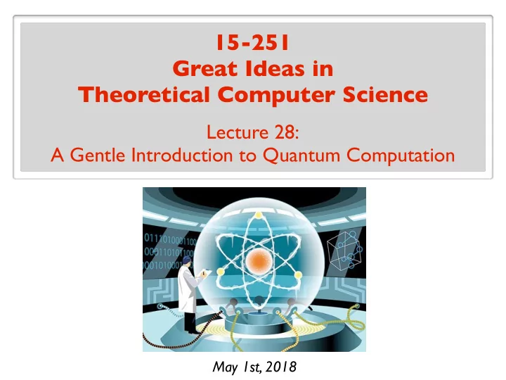
15-251 Great Ideas in Theoretical Computer Science Lecture 28: A Gentle Introduction to Quantum Computation May 1st, 2018
Announcements Please fill out the Faculty Course Evaluations (FCEs). https://cmu.smartevals.com
Announcements You can vote to eliminte 2 topics from the final exam: Stable Matchings Boolean Circuits NP and Logic (Descriptive Complexity) Transducers Presburger Arithmetic
Announcements The Last Lecture on Thursday Daniel Sleator Mor Harchol-Balter Ariel Procaccia Rashmi Vinayak Anupam Gupta Ryan O’Donnell
Announcements The Last Lecture on Thursday
Quantum Computation
The plan Classical computers and classical theory of computation Quantum physics (what the fuss is all about) Quantum computation (practical, scientific, and philosophical perspectives)
The plan Classical computers and classical theory of computation
What is computer/computation? A device that manipulates data (information) Usually Input Device Output
Theory of computation Mathematical model of a computer: (uniform) Turing Machines ~ Boolean Circuits
Theory of computation Turing Machines
Theory of computation Boolean Circuits 0 AND OR 1 AND NOT 1 AND 0 0 OR OR OR 1 OR 0 AND gates AND OR NOT
Theory of computation Boolean Circuits OUTPUT INPUT 0 AND OR 1 AND NOT 1 AND n bits 0 1 bit 0 OR OR OR 1 OR 0 AND Circuit n bits 1 bit (or m bits)
Physical Realization Circuits implement basic operations / instructions. Everything follows classical laws of physics!
(Physical) Church-Turing Thesis Turing Machines ~ (uniform) Boolean Circuits universally capture all of computation. Python Java, C, … TMs All types of computation
(Physical) Church-Turing Thesis Turing Machines ~ (uniform) Boolean Circuits universally capture all of computation. (Physical) Church Turing Thesis Any computational problem that can be solved by a physical device, can be solved by a Turing Machine. Strong version Any computational problem that can be solved efficiently by a physical device, can be solved efficiently by a TM.
The plan Classical computers and classical theory of computation Quantum physics (what the fuss is all about) Quantum computation (practical, scientific, and philosophical perspectives)
The plan Quantum physics (what the fuss is all about)
One slide course on physics Classical General Theory Quantum Physics of Relativity Physics
One slide course on physics Classical General Theory Quantum Physics of Relativity Physics String Theory (?)
Video: Double slit experiment http://www.youtube.com/watch?v=DfPeprQ7oGc Nature has no obligation to conform to your intuitions.
Video: Double slit experiment
2 interesting aspects of quantum physics 1. Having multiple states “simultaneously” e.g.: electrons can have states spin “up” or spin “down”: or | up i | down i In reality, they can be in a superposition of two states. 2. Measurement Quantum property is very sensitive/fragile ! If you measure it (interfere with it), it “collapses”. So you either see or . | up i | down i
It must be just our ignorance - There is no such thing as superposition . - We don’t know the state, so we say it is in a superposition . - In reality, it is always in one of the two states. - This is why when we measure/observe the state, we find it in one state. God does not play dice with the world. - Albert Einstein Einstein, don’t tell God what to do. - Niels Bohr
How should we fix our intuitions to put it in line with experimental results ?
Removing physics from quantum physics mathematics underlying quantum physics = generalization/extension of probability theory (allow “negative probabilities”)
Probabilistic states and evolution vs Quantum states and evolution
Probabilistic states Suppose an object can have n possible states: | 1 i , | 2 i , · · · , | n i At each time step, the state can change probabilistically. 1 What happens if we start at 2 state and evolve? | 1 i | 1 i | 2 i 1 1 Initial state: 1 4 3 2 | 1 i 1 | 3 i 4 | 2 i 0 | n i | 3 i 0 1 . . . | n i 0
Probabilistic states Suppose an object can have n possible states: | 1 i , | 2 i , · · · , | n i At each time step, the state can change probabilistically. 1 What happens if we start at 2 state and evolve? | 1 i | 1 i | 2 i 1 After one time step: 1 1 4 3 2 | 1 i 1 0 | 3 i 4 | 2 i 1 / 2 0 | n i Transition | 3 i 0 0 1 = Matrix . . . . . . | n i 1 / 2 0
Probabilistic states | 1 i 1 0 | 2 i 1 / 2 0 Transition the new state | 3 i 0 0 = (probabilistic) Matrix . . . . . . | n i 1 / 2 0 A general probabilistic state: p 1 p i = the probability of being in state i p 2 p 1 + p 2 + · · · + p n = 1 . . . ( ` 1 norm is 1) p n
Probabilistic states | 1 i 1 0 | 2 i 1 / 2 0 Transition the new state | 3 i 0 0 = (probabilistic) Matrix . . . . . . | n i 1 / 2 0 A general probabilistic state: p 1 p 1 | 1 i + p 2 | 2 i + · · · + p n | n i p 2 = 1 0 0 . . . 0 1 0 p n . . . . . . . . . 0 0 1
Probabilistic states Evolution of probabilistic states Any matrix that maps Transition probabilistic states to probabilistic states. Matrix We won’t restrict ourselves to just one transition matrix. K 1 K 2 K 3 π 0 − → π 1 − → π 2 − → · · ·
Quantum states p i ’s can be negative. p 1 p 2 . . . p n
Quantum states ( ’s are called amplitudes.) α i ’s can be negative. α i α 1 α 2 α 1 | 1 i + α 2 | 2 i + · · · + α n | n i = . . . α 2 1 + α 2 2 + · · · + α 2 n = 1 ( ` 2 norm is 1) α n ( α i can be a complex number) β 1 α 1 β 2 Unitary α 2 β 2 1 + β 2 2 + · · · + β 2 n = 1 = Matrix . . . . . . β n α n any matrix that preserves “quantumness”
Quantum states Evolution of quantum states Any matrix that maps Unitary quantum states to quantum states. Matrix We won’t restrict ourselves to just one unitary matrix. U 1 U 2 U 3 ψ 0 − → ψ 1 − → ψ 2 − → · · ·
Quantum states Measuring quantum states α 1 α 2 α 1 | 1 i + α 2 | 2 i + · · · + α n | n i = . . . α n α 2 1 + α 2 2 + · · · + α 2 n = 1 When you measure the state, α 2 you see state with probability . i i
Probabilistic states vs Quantum states Suppose we have just 2 possible states: and | 1 i | 0 i � � � 1 / 2 1 / 2 1 / 2 1 = 1 / 2 1 / 2 1 / 2 0 randomize a random state random state � � � 1 / 2 1 / 2 1 / 2 0 = 1 / 2 1 / 2 1 / 2 1 | 0 i ! 1 +1 2 | 0 i | 1 i 2 ✓ 1 ◆ ✓ 1 ◆ 2 | 0 i + 1 2 | 0 i + 1 1 1 2 | 1 i 2 | 1 i 2 2 4 | 0 i + 1 1 1 4 | 0 i + 1 4 | 1 i 4 | 1 i +
Probabilistic states vs Quantum states Suppose we have just 2 possible states: and | 1 i | 0 i √ √ 1 / � � √ − 1 / 1 / � 2 2 1 2 √ √ = √ 1 / 1 / 0 2 2 1 / 2 √ √ √ 1 / � � − 1 / � − 1 / 2 2 0 2 √ √ √ = 1 / 1 / 1 1 / 2 2 2 1 + 1 | 0 i ! p | 0 i | 1 i √ 2 2 ✓ 1 ✓ ◆ ◆ � 1 2 | 0 i + 1 1 2 | 0 i + 1 1 p p p p 2 | 1 i 2 | 1 i √ √ 2 2 � 1 2 | 0 i + 1 2 | 0 i + 1 1 = | 1 i 2 | 1 i 2 | 1 i +
Probabilistic states vs Quantum states Classical Probability To find the probability of an event: add the probabilities of every possible way it can happen
Probabilistic states vs Quantum states Quantum To find the probability of an event: add the amplitudes of every possible way it can happen, then square the value to get the probability. one way has positive amplitude the other way has equal negative amplitude event never happens!
Probabilistic states vs Quantum states A final remark Quantum states are an upgrade to: 2-norm (Euclidean norm) and algebraically closed fields. Nature seems to be choosing the mathematically more elegant option.
Recommend
More recommend
Explore More Topics
Stay informed with curated content and fresh updates.
