1 Enumeration Cont. How many different ways can we create a graph - PDF document
1 Enumeration Cont. How many different ways can we create a graph given a vertex set of size n ? Cayleys Formula states that with a vertex set of n there are n n 2 possible trees. Another way to think about it: the number of possible trees
1 Enumeration Cont. How many different ways can we create a graph given a vertex set of size n ? Cayley’s Formula states that with a vertex set of n there are n n − 2 possible trees. Another way to think about it: the number of possible trees is the number of spanning trees of complete graph. So how do we compute the number of spanning trees of a general graph? We can use a simple recurrence relation to do so. The number of possible spanning trees in a graph τ ( G ) is equal to the sum of the number of spanning trees of the graph with an edge removed τ ( G − e ) plus the the number of spanning trees of the graph with an edge contracted τ ( G · e ). An edge contraction involves combining the endpoints u, v of a given edge e into a single vertex, such that the new vertex has incident edges of all original edges of both u and v except for e . We can also use the adjacency matrix of G to compute the number of spanning trees through the matrix tree theorem . We form an n × n matrix Q as Q = D − A , where D is the diagonal matrix of degrees (similar to what we used to create the transition probability matrix when computing PageRank algebraically) and A is the adjacency matrix of G with loops removed. A matrix such as Q is also called a Laplacian matrix. Loops don’t affect the number of spanning trees. The number of spanning trees in G is then the determinant of Q with a row s and column t removed. See the book for a proof when s = t . 2 Graceful Labeling A graceful labeling of a graph is a labeling of all n vertices of a graph with unique labels from 0 . . . m , such that each of the m edges has a unique value computed as the difference between the labels of its endpoints. A graph is graceful if it has a graceful labeling. Ringel-Kotzig Conjecture : all trees are graceful. This is unproven, however, certain subsets of of trees have been proven to be. These include paths and caterpillar graphs . Caterpillar graphs are trees in which a single path is incident to or contains every edge in the graph. Hypercubes have also been proven to be graceful. 3 Minimum Spanning Tree Given an undirected and connected graph that has some numeric weight assigned to each edge, the minimum spanning tree problem seeks to create a spanning tree such that the sum of the weights selected for the edges of the spanning tree is minimized. We’re assuming the weights here are non-negative. There are two classical algorithms for this 1
problem. They include Krushkal’s algorithm and Prim’s algorithm. procedure Krushkal (Graph G = { V ( G ) , E ( G ) , W ( G ) } ) ⊲ W ( G ) is a numeric weight for each edge in E ( G ) V ( T ) ← V ( G ) ⊲ Spanning tree T will have all vertices of G E ( T ) ← ∅ ⊲ Edge set of T initially null sort W ( G ) and correspondingly E ( G ) by nondecreasing values in W ( G ) for all w, e ∈ W ( G ) , E ( G ) do if numComponents( T + e ) < numComponents( T ) then E ( T ) ← E ( T ) + e if numComponents( T ) = 1 then break return T Krushkal initializes the spanning tree T to include all vertices in the original graph G . A minimum weight edge is added as long as it reduces the number of components in T . The algorithm terminates once there is only a single component, i.e. T is now a spanning tree. procedure Prim (Graph G = { V ( G ) , E ( G ) , W ( G ) } ) ⊲ W ( G ) is a numeric weight for each edge in E ( G ) V ( T ) ← ∅ ⊲ Spanning tree’s vertices initially null E ( T ) ← ∅ ⊲ Edge set of T initially null V ( T ) ← randomSelect( V ( G )) ⊲ Randomly select one vertex from G while | V ( T ) | � = | V ( G ) | do e ← min( W ( u, v )) ∈ E ( G ) : u ∈ V ( T ) , v / ∈ V ( T ) ⊲ Minimum weight edge in G with only one vertex in T E ( T ) ← E ( T ) + e V ( T ) ← V ( T ) + v return T Prim initializes by randomly selecting a vertex in G and adding it to T . Iteratively, the minimum-weight edge between a vertex in T and a vertex not yet in T is added to T along with the associated vertex. The algorithm terminates when T has all vertices in G . 4 Shortest Paths Again, given an undirected and connected graph that has some numeric weight assigned to each edge, the shortest paths problem seeks to find the minimum distance between a vertex u and all other vertices v ∈ V ( G ). Distance here is defined as the sum of the weights along a u, v -path. A classic algorithm for computing these distances is Dijkstra’s algorithm. 2
procedure Dijkstra (Graph G = { V ( G ) , E ( G ) , W ( G ) } , vertex u ) ⊲ Finding all distances from u for all v ∈ V ( G ) do D ( v ) ← ∞ ⊲ Distances from u D ( u ) ← 0 S ← V ( G ) ⊲ Unvisited set while S � = ∅ do current ← min( D ( v ) , v ∈ S ) ⊲ Current vertex considered has minimum distance in unvisited set for all v ∈ N ( current ), where v ∈ S do w ← W ( current, v ) ⊲ Weight of edge between current and v if D ( current ) + w < D ( v ) then D ( v ) ← D ( current ) + w S ← S − current ⊲ Remove current from unvisited set return D The algorithm initializes all distances D ( v ) to infinity except for the root vertex u , which has distance zero. The algorithm as tracks an unvisited set of vertices, where on each iteration a vertex with the minimum distance from u is selected. All edges adjacent this vertex are examined, and if a distance from that vertex to a neighbor plus the distance from u the current vertex is less than what is currently stored in the distance array for u to the neighbor, the distance array is updated. After examining all neighbors, the vertex is removed from the unvisited set. The algorithm terminates once the unvisited set is empty. 5 Breadth-first Search A simple solution to the previous two problems for unweighted graphs can be accomplished with a breadth-first search traversal. For breadth-first search, we select our root vertex u and iterative visit all vertices one hop, two hops, three hops, etc. away from u that have not yet been visited. This creates a breadth-first search tree, which is a spanning tree as well as a tree containing paths of a minimum distance from u . Computationally, it’s easiest to track the parent of each vertex, where the parent is a neighbor of a distance closer to the root. E.g. the vertices one hop from the root have a distance value of one and a parent of the root. 3
procedure BFS (Graph G = { V ( G ) , E ( G ) , W ( G ) } , vertex u ) ⊲ u is the root for all v ∈ V ( G ) do D ( v ) ← ∞ ⊲ Distances from u P ( v ) ← − 1 ⊲ Parent in the BFS tree D ( u ) ← 0 P ( u ) ← u Q ← u ⊲ Queue for vertices to visit on current iteration Q n ← ∅ ⊲ Queue for next iteration while Q � = ∅ do for all v ∈ Q do for all w ∈ N ( v ) do if D ( w ) = ∞ then D ( w ) ← D ( v ) + 1 P ( w ) ← v Q n ← w swap( Q, Q n ) return D, P 4
Recommend
More recommend
Explore More Topics
Stay informed with curated content and fresh updates.


