1 Analysis of SNP data with R The data we will be working with here - PDF document

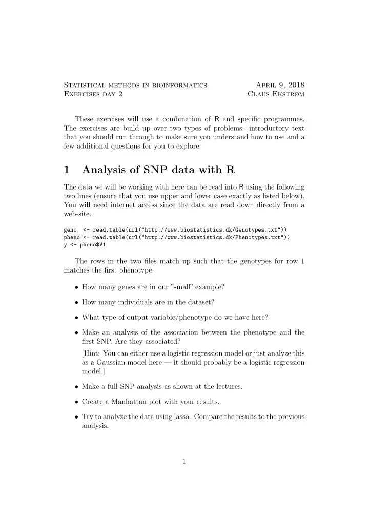
Statistical methods in bioinformatics April 9, 2018 Exercises day 2 Claus Ekstrøm These exercises will use a combination of R and specific programmes. The exercises are build up over two types of problems: introductory text that you should run through to make sure you understand how to use and a few additional questions for you to explore. 1 Analysis of SNP data with R The data we will be working with here can be read into R using the following two lines (ensure that you use upper and lower case exactly as listed below). You will need internet access since the data are read down directly from a web-site. geno <- read.table(url("http://www.biostatistics.dk/Genotypes.txt")) pheno <- read.table(url("http://www.biostatistics.dk/Phenotypes.txt")) y <- pheno$V1 The rows in the two files match up such that the genotypes for row 1 matches the first phenotype. • How many genes are in our ”small” example? • How many individuals are in the dataset? • What type of output variable/phenotype do we have here? • Make an analysis of the association between the phenotype and the first SNP. Are they associated? [Hint: You can either use a logistic regression model or just analyze this as a Gaussian model here — it should probably be a logistic regression model.] • Make a full SNP analysis as shown at the lectures. • Create a Manhattan plot with your results. • Try to analyze the data using lasso. Compare the results to the previous analysis. 1

2 Find linkage disequilibrium (LD) blocks The following text explains how to make a heat map in R . Heat map plots are used to visualize data from a two-dimensional array using colors to indicate the values in the array. In R , the function heatmap plots a heat map, and it requires a numeric matrix as its first argument. There are several formulas for computing linkage disequilibrium between two genes. A simple measure that is fast to compute and easy to interpret is the correlation coefficient. cor computes the correlation matrix for all pairwise correlations. • Read in the hapmap1 and qt data from the web page (see instruction in the slides). • Compute the correlation matrix for the first 100 genes/SNPs. • Use heatmap(x, Rowv=NA, Colv=NA) ( x is the matrix of correlation values computed above). What do you see in the graph? • What happens if you do not include the arguments Rowv=NA, Colv=NA ? The color scheme of the heat map plot can be set with the col option. By default it uses heat colors obtained from the heat.colors function, but that can be changed to give other color schemes. If the options ColSideColors and RowSideColors are provided, they should contain a vector of color names for a horizontal/vertical side bar that annotates the columns and rows of the data matrix, respectively. This can be used to indicate known groupings by color code as shown below. 3 Population admixture The researchers are nervous that there is population admixture in the data. This essentially means that the full population in reality contains two or more ”hidden” sub-populations. • Why is population admixture a potentially big problem? We can use principal component analysis based on all SNPs to produce a combined measure (of the SNPs). If there is population substructure then the allele frequencies are likely to be different among different sub-populations and across many SNPs and this effect is likely to be captured by the principal component since they are computed regardless of the outcome. 2

• Read in the hapmap1 and qt data from the web page (see instruction in the slides). • Make a full analysis where you also take potential population structure into account. How does this change the results? [ Hint: compute a principal component or two and check if they con- tribute anything to the analyses. ] • Which markers should ideally be used for the principal components? 4 Rare variants We want to see if there is any reason to consider a burden/SKAT test in order to find association between rare variants and the outcome. • Compute the minor allele frequency for each of the genes. What is the distribution of allele frequencies? You can use the colMeans function to compute the mean of the columns in the genotype data. • For each of the rare SNPs: Identify the SNPs found to be in the same clusters using the heatmap from above and make a simple burden test for each of the clusters identified. An example of this can be analyzed in R as follows (needs to be modified): > library("lme4") > # Include, say, V6 and V7 as random variable > y <- pheno$V3 > fullmodel <- lmer(y ~ 1 + (1|V6) + (1|V7), data=geno2, REML=FALSE) > smallmodel <- lm(y ~ 1, data=geno2) > logLik(fullmodel) > logLik(smallmodel) • How should we compare the results? 5 ”Heritability” In this exercise we will try to estimate the proportion of variance explained. To do this we will use the lmekin function from the coxme package. • We should start by computing the allele frequencies for each of the SNPs. Use the colMeans function. 3

• The mean of each SNP is 2 p where p is its allele frequency, and it has a � standard deviation of 2 p (1 − p ). Standardize the values for each gene by subtracting the correct mean and dividing by its standard deviation. Call the result W in R . See the code below for inspiration. • Run the code MAF <- 1-colMeans(geno2)/2 # Minor allele frequency W <- t((t(geno2)/2 - MAF)/sqrt(2*MAF*(1-MAF))) N <- length(y) A <- tcrossprod(W) / ncol(geno2) library(coxme) id <- 1:N res <- lmekin(y ~ 1 + (1|id), varlist=list(id=A)) The first couple of lines compute the correlation matrix we should use for the calculations. The last line fits the model. • Explain what goes on in the code above. • Estimate the proportion of variance explained. 6 plink This exercise is to try the software program plink. You need to download and install that before you can run the exercise. plink is super versatile and has many more options than what we can consider here. Instead we will try to make small extensions to the analyses we made above. • Download the plink program from http://zzz.bwh.harvard.edu/plink/download.shtml and install it. The plink executable file should be placed in either the current working di- rectory or somewhere in the command path. All commands involve typing plink at the command prompt followed by a number of options (all starting with -option ) to specify the data files / methods to be used. plink needs two standard files: a ped-file and a map-file. • Check the files and make sure you understand their formats. The map file contains chromosome number, the SNP name, the position in mor- gans on the chromosome, and the position in base pairs on the chro- mosome. 4

• Type plink --noweb --file hapmap1 and look at the output. It takes two files (a ped file and a map file) as input. They can be down- loaded from the website. • Type plink --noweb --missing --file hapmap1 and look at the out- put. What information is contained in the missing files. • Type plink --noweb --freq --file hapmap1 and look at the out- put. What information is contained in the frequency files. How does the results compare to the results you computed manually earlier in R? • Type plink --noweb --assoc --file hapmap1 and look at the out- put. What information is contained in the association files. • Type plink --noweb --assoc --adjust --file hapmap1 and look at the output. What information is contained in the adjusted associa- tion files. 5